Simply

Modeling

Introduction

The modelling of synthetic biology systems is vital in the design of genetic circuits. To be able to construct sequences of increasing complexity – on the scale of the natural networks already present in the bacteria it is necessary develop satisfactory computational tools to predict and mimic the behaviour of the system.
To predict the output of our genetic circuit we created a single cell model for our circuit. The effect of transcription regulators on gene expression was assumed to follow Hill equation kinetics, with first order kinetics for the degradation of the proteins/enzymes formed. The models were created in MATLAB.

Phosphatase Amplification Circuit

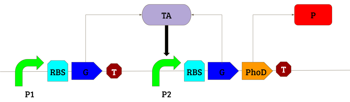
The positive feedback amplification circuit shown above was used in our study to obtain an amplified production of our gene of interest in presence of an inducing chemical. For more details on the parts used in the circuit please visit the Design page.

Deterministic Model

The deterministic model involves creating a series of differential equations which are solved simultaneously using certain initial conditions. The differential equations were obtained by performing a mass balance for each protein being expressed. For the transcriptional activator (‘TA’):

It is formed by gene expressed by promoter P1 which is induced by the an inducer ‘I’ \[ Rate\ of\ formation\ of\ TA\ through\ P1=\frac{V_{{max}_I}*{[I]}^{n_I}}{k_I^{n_I}+{[I]}^{n_I}} \]
It is formed by gene expressed by promoter P2 which is induced by itself ‘TA’ \[ Rate\ of\ formation\ of\ TA\ through\ P2=\frac{V_{{max}_{TA}}*\ {[TA]}^{n_{TA}}}{k_{TA}^{n_{TA}}+{[TA]}^{n_{TA}}} \]
It is degraded \[ {Rate\ of\ degradation\ of\ TA=\delta{}}_{TA}[TA] \]

By a mass balance, the overall rate of change of the concentration of the transcriptional regulator is thus given by: \[ \frac{d[TA]}{dt}=\frac{V_{{max}_I}*{[I]}^{n_I}}{k_I^{n_I}+{[I]}^{n_I}}+\frac{V_{{max}_{TA}}*\ {[TA]}^{n_{TA}}}{k_{TA}^{n_{TA}}+{[TA]}^{n_{TA}}}-{\delta{}}_{TA}\left[TA\right]+{\alpha{}}_{TA} \]
Similarly for the reporter protein RFP (‘R’):

It is formed by gene expressed by promoter P2 which is induced by the transcriptional regulator ‘TR’ \[ Rate\ of\ formation\ of\ R\ through\ P2=\frac{V_{{max}_{TA}}*\ {[TA]}^{n_{TA}}}{k_{TA}^{n_{TA}}+{[TA]}^{n_{TA}}} \]
It is degraded \[ {Rate\ of\ degradation\ of\ R=\delta{}}_R[R] \]

By a mass balance, the overall rate of change of the concentration of the transcriptional regulator is thus given by: \[ \frac{d[R]}{dt}=\frac{V_{{max}_{TA}}*\ {[TA]}^{n_{TA}}}{k_{TA}^{n_{TA}}+{[TA]}^{n_{TA}}}-{\delta{}}_R\left[R\right]+{\alpha{}}_R \]

The resulting trend obtained through the deterministic model is shown below:

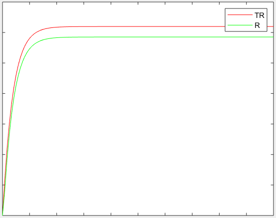
On solving the above two differential equation simultaneously, with the following initial conditions, we get a curve as shown below:

Stochastic model

The deterministic model takes into account only the initial condition based on which it gives an output curve with respect to time. A more accurate way of representing a biological system is through a stochastic model which accounts for the “randomness” in the biological systems. The stochastic model was built based on the Gillespie algorithm[2]. In this model, each possible step was given a probability and then a particular step was selected at random and changes made to the current state of the system. The different steps taken were:

TA is produced through promoter P1
TA is produced through promoter P2
TA is degraded
R is produced through promoter P2
R is degraded

The resulting trend obtained through the stochastic model is shown below:

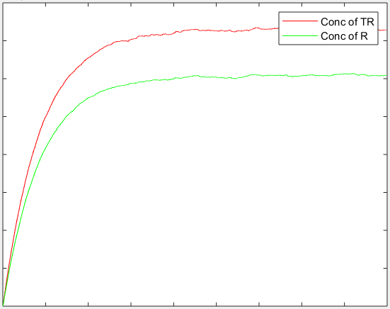
Both the above models are qualitative in nature at this stage. This is because we do not as yet know which inducible promoter will be used and hence cannot estimate the parameters for it .The amplification circuit is known to produce a higher concentration of the target protein than simple expression of the protein – and the change in concentration of the protein with time is similar to the trend we have obtained.[3] Once we are able to identify the promoters and components of the circuit being used, we will be able to plug in the parameter values to this model and quantify it.

Qualitative model of potential application of project

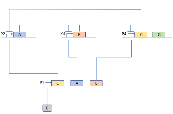
The above circuit is based on the standard three node repressilator circuit.[4] It has been modified so that the oscillations only take place in presence of ‘E’, i.e., it is an oscillatory circuit with an external switch to start/stop the oscillations. A, B and C are proteins that successively repress the next promoter. ‘G’ is our required product protein. The circuit is designed so as to ensure that there is no G produced in absence of E, but we get an oscillating output of G in presence of E. Since we expect an oscillatory output, we cannot simply solve the differential equations using initial conditions as this gives a Michaelis-Menten type curve (given the nature of the equations used). So we created a stochastic model for this circuit. The steps considered for the stochastic model are shown below:

For A:

A is produced by promoter P1 which is repressed by E \[ rate\ of\ formation=\ \frac{V_{{max}_E}*\ k_E^{n_E}}{k_E^{n_E}+{[E]}^{n_E}} \] (**above equation based on the Hill equation)
A is produced by promoter P2 which is repressed by C \[ rate\ of\ formation=\ \frac{V_{{max}_C}*\ k_C^{n_C}}{k_C^{n_C}+{[C]}^{n_C}} \]
A gets degraded \[ rate\ of\ degradation=\ {\delta{}}_A[A] \]
A is produced due to its basal transcription level (leakage rate) \[ rate\ of\ formation=\ \alpha_A \]

For B:

B is produced by promoter P1 which is repressed by E \[ rate\ of\ formation=\ \frac{V_{{max}_E}*\ k_E^{n_E}}{k_E^{n_E}+{[E]}^{n_E}} \]
B is produced by promoter P3 which is repressed by A \[ rate\ of\ formation=\ \frac{V_{{max}_A}*\ k_A^{n_A}}{k_A^{n_A}+{[A]}^{n_A}} \]
B gets degraded \[ rate\ of\ degradation=\ {\delta{}}_B[B] \]
B is produced due to its basal transcription level (leakage rate) \[ rate\ of\ formation=\ \alpha_B \]

For C:

C is produced by promoter P1 which is repressed by E \[ rate\ of\ formation=\ \frac{V_{{max}_E}*\ k_E^{n_E}}{k_E^{n_E}+{[E]}^{n_E}} \]
C is produced by promoter P4 which is repressed by B \[ rate\ of\ formation=\ \frac{V_{{max}_B}*\ k_B^{n_B}}{k_B^{n_B}+{[B]}^{n_B}} \]
C gets degraded \[ rate\ of\ degradation=\ {\delta{}}_C[C] \]
C is produced due to its basal transcription level (leakage rate) \[ rate\ of\ formation=\ \alpha_C \]

For G:

G is produced by promoter P4 which is repressed by B \[ rate\ of\ formation=\ \frac{V_{{max}_B}*\ k_B^{n_B}}{k_B^{n_B}+{[B]}^{n_B}} \]
G gets degraded \[ rate\ of\ degradation=\ {\delta{}}_G[G] \]
G is produced due to its basal transcription level (leakage rate) \[ rate\ of\ formation=\ \alpha_G \]

The resulting trend obtained for the given model in response to a step input to the concentration of the external inducer E is shown below:
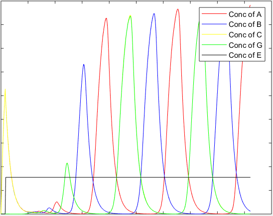
Like the amplification circuit, this model is also qualitative in nature as the exact promoters being used are not known and hence their parameter values are unknown. This circuit is more sensitive to variations in parameters than the amplification circuit. However, the general nature of the curve obtained shows that oscillations do start when the external inducer is added to the system.

References

[1] Jennifer A.N. Brophy and Christopher A. Voigt, “Principles of Genetic Circuit Design”, Nat. methods, May 2014
[2] “Systems Biology” by Uri Alon
[3] Goutam J Nistala, Kang Wu, Christopher V Rao, Kaustubh D Bhalerao, ‘A modular positive feedback-based gene amplifier’, Journal of Biological Engineering, 2010
[4] Michael B. Elowitz & Stanislas Leibler, ‘A synthetic oscillatory network of transcriptional regulators’, Nature vol. 403, 2000