Team:Imperial College/Model


Modelling

Diffusion modelling
Analytical Evaluation
We wanted to perform the initial evaluation for the concentration profile by hand to ensure we knew every assumption made in its entirety, and to maximise our understanding of the system. We did not want to simply use numerical modelling software without first understanding the key concepts and limitations within the system to be able to identify aberrant results and unjustified assumptions.
The analytical model is a reworking of a system solved by Bell, Seelanan and O'Hare (2017). We initially modelled the diffusion of the chemical species away from the electrode by treating the electrode as a disc source with a constant flux of the redox molecule across its interface with the medium. We were able to use a pure diffusion model (without systematic drift) because the high ionic concentration of the medium shields any electric fields around the electrodes to a lengthscale of 0.8nm. We then assumed that the agar medium itself was not generating additional molecules, and therefore that the only source of said molecules was the disc electrode. This assumption, combined with the conservation of species, allows us to describe the concentration of the species within the agar with the partial differential equation known as the Laplace equation. The Laplace equation describes diffusion processes in the limit of no time-dependence (the steady state reached at infinite time).
The radially symmetric nature of the problem (the problem looks the same from any angle, as the electrode is a disc, not a rectangle or any other shape) allows us to use the 2D axisymmetric form of the Laplace equation, rather than the full 3D form, which makes solving the problem easier.
Due to the slow speed of diffusion, and the square root proportionality between time and diffusion distance, we assumed that the agar plate was arbitrarily deep, and that the concentration of the species tended to 0 as depth (z) increased. This can also be conceptualised as the diffusion “front” not reaching the bottom of the plate within the timescales that we are interested in. This assumption was also applied in the radial direction (ie the diffusion front does not reach the edge of the agar plate within the timescales that we are measuring within). This assumption was later confirmed through the use of Comsol modelling. We also constrained the problem to positive values of z, meaning that no molecules can leave the agar through its top surface. We also assumed that the chemical species analysed would not adsorb onto, or otherwise interact with, the agar medium.
The full mathematical solution for the problem, as well as the justification for the assumption that the molecules are only transported by diffusion, is given in the appendix
However, we shall say here that the problem was formulated in cylindrical coordinates (again due to the radially symmetric nature of the problem), and non-dimensionalised both to simplify working and to generalise the problem to any desired scales (scales here meaning length scale of the problem and scale of diffusion, normalised for diffusion constant and flux through the electrode). The scalings are given below.

Formula 1. Scalings used to non-dimensionalise the analytical model
The problem was evaluated analytically and by hand up until the last step. That last step involved the evaluation of a complicated infinite integral, which was non-trivial. However, because the integrand tends to 0 as the variable tends to infinity, use of numerical integration in this case was justified to give the solution for the dimensionless concentration profile.
Figure 2. Visualisations of the integrand, or the distribution in Hankel space, for the analytic model
The exact magnitude of concentration for a given species at a specific flux can be found through simply reinserting the diffusion coefficient for that species. Interestingly, the diffusion coefficients for the species of interest are all reasonably similar, and so give reasonably similar results. Despite this, a wider range of diffusion coefficients was tested (between 5e-10m^2s^-1 and 1e-9m^2s^-1) to account for any differences from literature value due to interactions with the agar medium, or differences due to molecular interactions within the solution.
Observing the scalings for the non-dimensionalised problem, it can be seen that the lengthscale over which the concentration decays towards its bulk value is directly proportional to the electrode radius, and therefore scales linearly with it. The concentration at any given point is directly proportional to the flux through the electrode, and inversely proportional to the Diffusion coefficient. The half-maximal width of the concentration profile is as wide as 1.145 electrode diameters, which confirms the feasibility of generating spatially resolved regions of oxidising or reducing environment, with the resolution limited only by the electrode radius, which can be considered an engineering parameter. For a 2mm radius electrode, it can be seen that the concentration drops to below a quarter of its peak magnitude by 6mm from the centre, and below a sixth of its peak magnitude by 8mm. These miniscule concentrations would be easily negated by the effect of an electrode of opposite polarity centred 8mm from the centre of the first, whilst still bringing the two electrode’s regions of influence close enough together for image formation. Thus, 2mm radius electrodes, with centes spaced 8mm from each other, were selected for use in the PCB. It should be noted that, for a patterning application, electrode spacing at a given electrode size is a tradeoff between pixel distinction and the percentage of a surface under direct influence of an electrode. The engineer should attempt to maximise coverage in order to minimise the number of cells that are not driven hard into either ‘off’ or ‘on’.
Figure 3. Analytic concentration profile for 2mm radius electrode
Figure 4. Profiles for different diffusion coefficients, showing its behaviour as a scaling factor in steady state
Figure 5. Concentration distributions throughout the volume of interest
Numerical studies with Comsol Multiphysics
Comsol is a very high-level Computer-aided design (CAD) tool, which supports the analysis of many types of problems with wide-ranging physics, and the coupling of different physical interfaces together to compute intricate and complicated problems. It has built-in geometry and meshing tools, which allow the user to create model geometry in-package, without the need of external CAD software, and was therefore perfect for performing our simulations.
The manual calculation of the diffusion profile, although useful, is confined to steady state, and cannot provide the same level of tunability as a model developed in a dedicated simulation software package such as Comsol. Building a model in Comsol allowed us to check the results of the analytical calculations, to observe the evolution of the concentration profile over time, and to quickly and easily analyse different geometries and test the assumptions made when formulating the analytical problem.
This model was constructed in order to test assumptions used in the analytical solution, specifically the assumptions that the diffusion “front” would not reach the edges of the plate within the relevant timescale. To do this, we used a time-dependent study with the 2D axisymmetric geometry pictured below, with the disc positioned flush to the surface.
Figure 6. Basic 2D axisymmetric geometry, where the disc electrode (small circle) is flush to the surface. The "wedge" cut out of the image allows a visualisation of the concentration profile as a function of depth.
Figure 7. Volumetric concentration distribution after 20 minutes
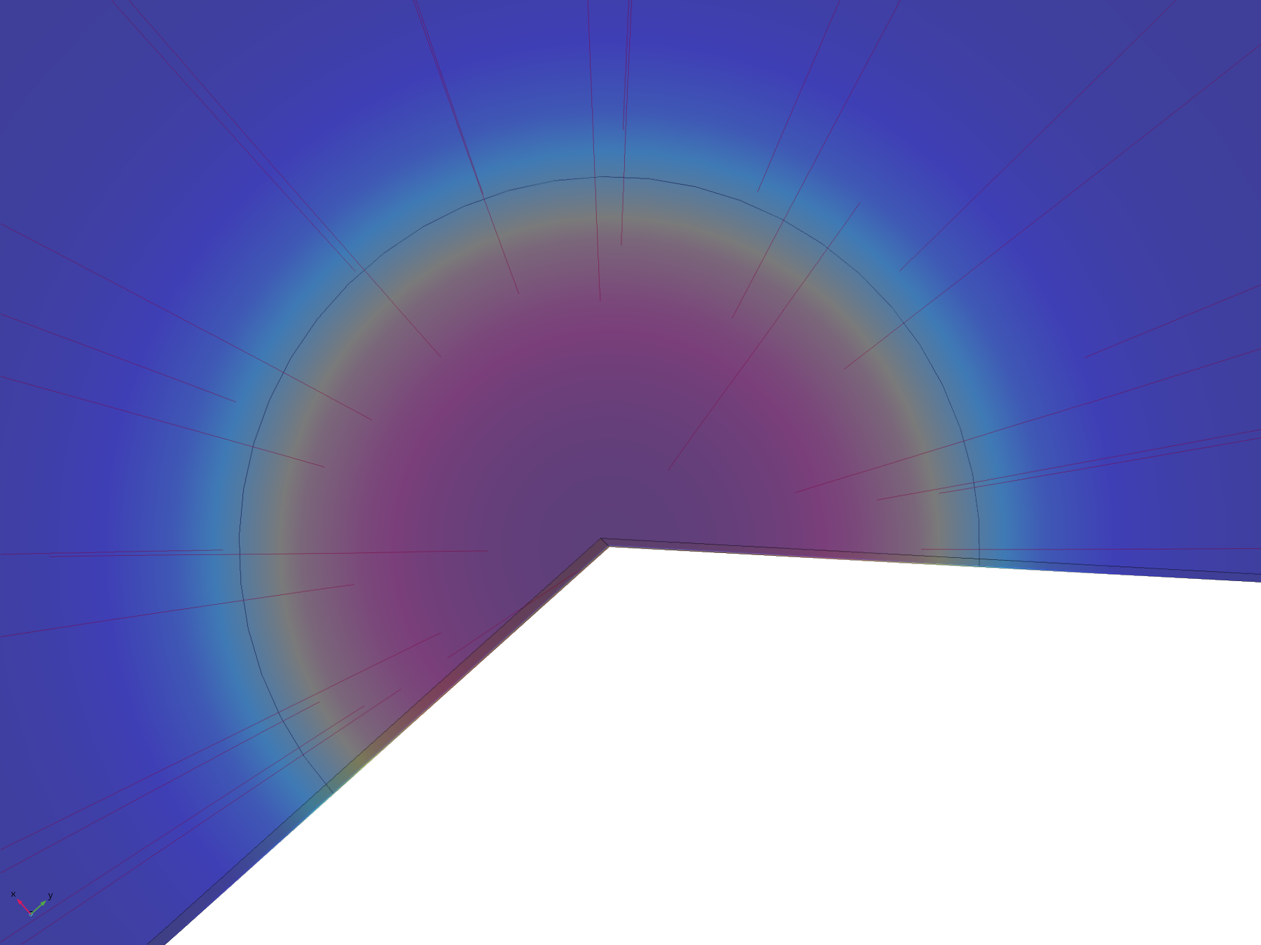
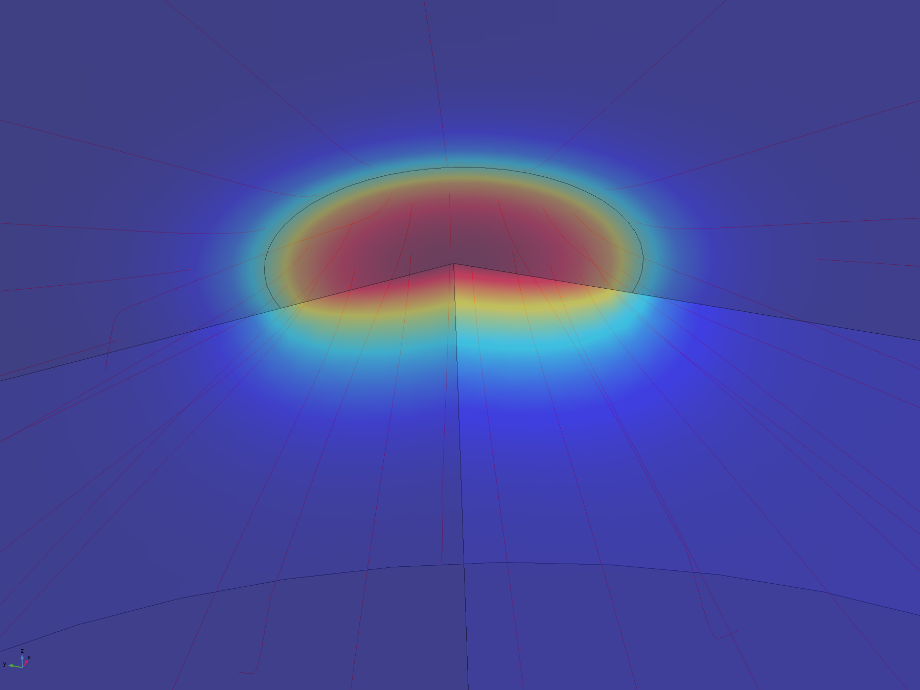
Figure 8. Flux lines showing the paths of diffusion from the electrode surface
From this model, we can conclude that the assumptions in the analytical solution regarding the diffusion “front” are valid, and that it is valid to treat the dish in the analytical solution as both arbitrarily deep and wide. Additionally, it is reasonable to think that localised oxidised or reduced volumes can be induced in the agar plate in a period of 20 minutes by the use of electrodes, which was confirmed experimentally.
When a manufacturer produces a PCB with pads on the underside, such as the one we ordered, the pads are plated, and then the underside of the PCB lacquered. This means that the actual surface of the pad is slightly recessed from the surface of the rest of the PCB. Therefore, we wanted to test how a small recession such as this would affect the concentration profile around the electrode. We again used 2D axisymmetric geometry, shown below, where the electrode disc is the top surface of the recessed cylinder.
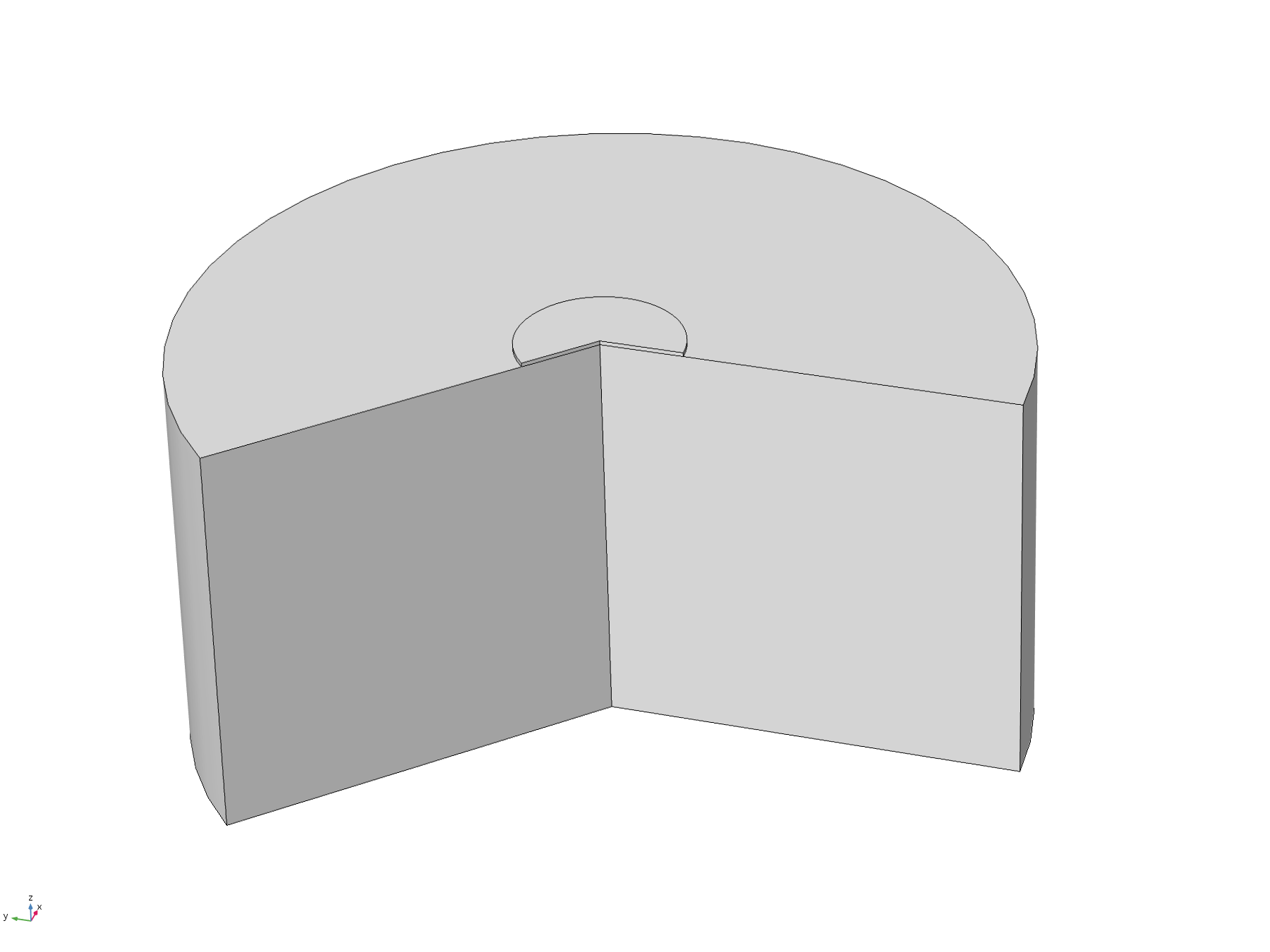
Figure 9. 2D axisymmetric geometry where the disc electrode (small circle) is recessed from the surface. The "wedge" cut out of the image allows a visualisation of the concentration profile as a function of depth.
Figure 10. Animation showing the behaviour of the concentration profile for different recession depths, between 1μm and 0.1mm
The flux lines emanating from the electrode in this model show how the recession, and hence the constriction of flux, adversely affect the efficiency of molecular transport. Comparing the flux line plots to those of the non-recessed model, it can be seen how they are significantly less uniform across the electrode, and cluster around its edge, as this is where the majority of the molecular flux occurs. This can also be seen in the lack of divergence of the central flux lines; molecules diffusing from the centre of the electrode can only diffuse downwards.
Figure 11. Flux lines showing diffusion paths from a recessed electrode
It should be noted that the decreased diffusive flux into the wider environment is not necessarily a bad thing, as although it limits the volume a particular electrode can affect, it increases the sharpness of the concentration profile (and hence gives a sharper on/off transition for induced cells at the boundary), and increases the concentration directly underneath the electrode, resulting in greater fold induction of any electro-inducible organisms in this region. Indeed, the magnitude of recession of electrodes within their mounting could be approached as an engineering specification, with a smaller recession resulting in wider but less well-defined fields of influence, and a larger recession resulting in smaller, sharper and more highly induced fields of influence.
Figure 12. Animation showing the concentration profiles across both the basic and recessed geometries, specifically the significant difference between the basic geometry and 1μm recession
Transcription-Translation Modelling
In order to better understand the system we are engineering, we constructed a deterministic transcription-translation model of the gene circuit using ordinary differential equations in Matlab. This model allowed us to explore the dynamics of the system, to better understand the parameters that the system would be sensitive to, to use curve fitting tools to estimate unknown parameters, and to check whether the constructs were behaving as expected.
Using parameters from literature, we constructed a model consisting of 4 coupled ODEs: one for transcription of soxR, one for translation of soxR, one for transcription of GFP, and one for translation of GFP. SoxR production was modelled as constitutive, as there was insufficient evidence in literature to support feedback control of the transcription of soxR. The binding of soxR to its promoter was modelled using the phenomenological transfer function given below. This transfer function has the effect of combining both the repressive and activatory modes of Hill functions into one, to account for the binding of both oxidised (activatory) and reduced (repressive) soxR molecules. There was no clear data to be found regarding the cooperativity of the soxR transcription factor; however, it is known that soxR forms dimers, so the maximum cooperativity is constrained at 2. Therefore, we decided to estimate the cooperativity as that of the dimeric tetR transcriptional regulator. TABLE Parameter Value Source
Formula 2. Transfer function describing SoxR promoter activity as a function oxidised and reduced SoxR
Formula 3. Full governing system for the Pixcell construct

Because Pyocyanin oxidises SoxR directly, we assumed that the oxidation of SoxR by Pyocyanin was fast compared to the timescales of the biological processes in the model, which are limited by the diffusion of large biological complexes. We therefore modelled the quantities of oxidised and reduced SoxR as instantaneously created from the total available pool of soxR, splitting the pool in the following way.
Formula 4. Proportions of oxidised and reduced SoxR as a function of Pyocyanin concentration

Table 1. Known model parameters and their sources
| Parameter | Description | Value | Unit | Source |
|---|---|---|---|---|
| Nplasmid | pMB1 ORI | 15 | 1 | (Morgan, 2018) |
| PpsoxS | Promoter strength of psoxS |
5.8 x 10^-3 | 1 | Calculated from average mRNA molecules per cell in E.coli, and the average half-life |
| Kox | Dissociation constant of Oxidised SoxR |
4.5 x 10 ^-10 | M | (Chen et al., 2018) |
| Kred | Dissociation constant of Reduced SoxR |
1.1 x 10 ^-10 | M | (Chen et al., 2018) |
| dmRNA-GFP | Average degradation rate of mRNA in E.Coli based on half-life |
2.5x10^-3 | 1/s | (Chen et al., 2018) |
| rbsGFP | RBS strength of GFP | 0.183 | 1/s | RBS strength calculator |
| Dgfp | degedration rate of GFP | 6.9X10^(-5) | (Halter et al., 2018) |
|
| SoxR @SS | Steady-state soxR in wild-type species |
75 | 1 | (Pomposiello and Demple, 2018) |
| n | Hill coefficient for TetR | 1.6 | 1 | (Ahn et al., 2018) |
Curve Fitting
For every model we wished to fit to data, we developed an objective function to minimise the square difference between the model and the experimental data by varying its parameters. We then used optimisation algorithms to find the optimum parameter set.
Most notably, this method of curve fitting was used to estimate parameters for the reaction between Pyocyanin and SoxR, which were unknown, as well as the basal expression, the GFP:RFU scale of the measurements, and the degradation rate of GFP, given the transcription/translation rates sourced from literature.
In order to utilise the entire available dataset, rather than merely the steady state GFP values for each Pyocyanin concentration, we constructed an objective function that could generate ODE plots. The reasoning behind using this more complicated strategy is as follows.
The steady state GFP reading can be computed using Formula 5 below. This is done by assuming that the system has been left for a long time and has settled, so that no quantity within the system is varying with time. Thus, all derivative terms in the model are zero, and so can be rearranged and combined together into one equation. Observing this steady state equation, it can be seen that there is orthogonality in all of the parameters in Table 2, besides the Scale and the degradation rate of GFP; a twofold increase in the Scale parameter can be compensated for by a twofold increase in the GFP degradation rate. However, the same is not true in the time-dependent model. It can be seen from Figures 12 and 13 that a twofold increase or decrease in these parameters leads to a differing transient response, and the same steady state response. Thus, an objective function that utilises transient data can fit both the GFP degradation rate and the GFP:RFU scale simultaneously.
Formula 5. Steady State GFP as a function of Pyocyanin

Table 2. Parameters to be fitted, with their descriptions
| Parameter | Description |
|---|---|
| Scale | Scaling to normalise RFU to number of GFP molecules |
| K | Concentration of oxidised Pyocyanin that leads to half of the soxR molecules being oxidised and half reduced |
| m | Stoichiometry of the reaction between Pyocyanin and soxR |
| Basal | Basal (leaky) expression of GFP |
| dGFP | Untagged degradation rate of GFP |
| dGFP_tagged | Degradation rate of degradation tagged GFP |
| Delay | Delay in cellular response to oxidising conditions |
Figure 12. Time-dependent curves show the non-equivalence of parameters
Figure 13. Differential transient behaviour highlighted by the removal of basal expression
It should be noted that, due to the steady state nature of the soxR dynamics in the fitted data, we can remove the ODEs describing soxR transcription and translation in order to decrease the significant computational cost associated with running many ODE solvers for each optimisation iteration. The governing equations to which the optimiser is fitting are then given below.Formula 6. Reduced set of equations to which are used by the optimisation algorithms to fit experimental data

Convergence of optimisation algorithms is of vital importance, and plotting the norm of the residuals (ie the dataset-wide error of the model) can be qualitatively very informative. An optimisation problem can be said to have converged if the norm of the residuals tends towards a certain value, at which the parameters allow the model to best fit the data. It should be noted that “best fit” is a misnomer; in practice, it can be very difficult to find a global minimum for the objective function, and so the computer can only find the best possible parameters close to the region it starts within. It can be seen from Figure 14 that convergence is obtained, and from Figure 15 that a reasonable fit of the data is achieved.
Figure 14. Convergence of model utilising the entire available dataset
Figure 15. Model function with fitted parameters compared to experimental data
However, upon inspection of the residual plot, below, it can be seen that there is noticeable patterning; there are regions which are consistently above or below zero. For a good model fit, the residuals should be randomly distributed about zero.
Figure 16. Dataset-wide plot of the residuals of the fitted model, showing undesirable clustering in their distribution
One noticeable feature of the residual plot is the overestimation of GFP expression at high Pyocyanin concentrations. Upon observation of the OD600 data (LINK TO OD600), it can be seen that, for Pyocyanin concentrations for 10μM and above, cell growth is significantly hindered. Although the model normalises for cell number, this lower OD600 is a sign of struggling cells, which activate stress pathways and downregulate non-essential genes, such as the synthetic construct. Therefore, the fit, and therefore the accuracy of extracted parameters, can be improved by omitting this data. Observing the convergence of the fitting algorithm for data up to 5μM, it can be observed that the norm of the residuals is drastically reduced. This signifies a better fit to the data. Note that this does not necessarily mean a better model, but is a useful measure nonetheless.
Figure 17. Convergence of the model for healthy cell data, noting the improvement of fit
Figure 18. Model function with parameters fitted to healthy cell data, compared to experimental data
Figure 19. Healthy cell model residual plot, noting reduced clustering
Observing the plot of the residuals for the reduced dataset, additional patterning can be seen in low time points.In order to account for this bias, data could be normalised and then fitted. For example, in the plots below, the average of the first six data points are subtracted uniformly from the data. Although this provides a small reduction in the value of the norm of the residuals upon model convergence, the fit is not markedly improved, and the residuals show higher clustering than before the normalisation. Thus, we concluded that the model cannot be easily normalised without significantly altering the data to improve the fit, which would invalidate the model and destroy any predictive power it might have. We therefore conclude that our best estimates of the parameters are found by fitting the model to the unaltered, healthy cell data.
Figure 20. Convergence for healthy cells, normalised to account for correlation between initial fluorescence and Pyocyanin concentration
Figure 21. Model fit for healthy cells, normalised for initial variable bias
Figure 22. Plot of residuals for normalised healthy cell data, noting higher clustering than the non-fitted group
The fitted parameters returned by the curve fitting regime are given in the table below.
| Parameter | Description |
|---|---|
| Scale | Scaling to normalise RFU to number of GFP molecules |
| K | Reciprocal of the concentration of oxidised Pyocyanin that leads to half of the soxR molecules being oxidised and half reduced |
| m | Stoichiometry of the reaction between Pyocyanin and soxR |
| Basal | Basal (leaky) expression of GFP |
| dGFP | Untagged degradation rate of GFP |
| dGFP_tagged | Degradation rate of degradation tagged GFP |
| Delay | Delay in cellular response to oxidising conditions |
Several interesting observations can be made from these estimated parameters. The basal expression fitted, although high, is not exactly unexpected due to the leakiness of the system, and could be a reasonable approximation for the real value. The untagged degradation rate for GFP is within 5% of the literature value, which, although interesting, cannot be taken as a direct measure of quality of the model due to the noise in the data, and the inherent tolerances and context dependencies of any metabolic parameter. The degradation rate of the tagged GFP was significantly slower than expected. To check this, the steady-state models are plotted against the final timepoint from the data. This model suggests that the degradation tag only increases the degradation rate by approximately a factor of 1.2, not by the expected factor of 8 (Tschirhart et al. 2017). On the basis of this unexpected result, the construct was sent for sequencing, and a mutation was confirmed within the degradation tag. It was decided, however, to keep using the mutated sequence, as it provided a good balance between reducing background and still retaining a measurable fluorescence when induced.
Figure 23. Plot of model fits for tagged and untagged constructs at steady state
Analytical Modelling Guide
References
- Ahn, S., Tahlan, K., Yu, Z. and Nodwell, J. (2018). Investigation of Transcription Repression and Small-Molecule Responsiveness by TetR-Like Transcription Factors Using a Heterologous Escherichia coli-Based Assay.
- Bell, C., Seelanan, P. and O'Hare, D. (2017). Microelectrode generator–collector systems for electrolytic titration: theoretical and practical considerations. The Analyst, 142(21), pp.4048-4057.
- Chen, H., Shiroguchi, K., Ge, H. and Xie, X. (2018). Genome-wide study of mRNA degradation and transcript elongation in Escherichia coli.
- Halter, M., Tona, A., Bhadriraju, K., Plant, A. and Elliott, J. (2018). Automated live cell imaging of green fluorescent protein degradation in individual fibroblasts.
- Kobayashi, K., Fujikawa, M. and Kozawa, T. (2018). Binding of Promoter DNA to SoxR Protein Decreases the Reduction Potential of the [2Fe–2S] Cluster.
- Morgan, K. (2018). Plasmids 101: Origin of Replication. [online] Blog.addgene.org. Available at: https://blog.addgene.org/plasmid-101-origin-of-replication [Accessed 18 Oct. 2018].
- Pomposiello, P. and Demple, B. (2018). Redox-operated genetic switches: the SoxR and OxyR transcription factors.


