Team:Oxford/Model/Frequency-Domain-Analysis
Frequency Domain Analysis
Description
The Frequency domain analysis is essentially a way of looking at the same problem from a different perspective. Here, we try to look at the model in a complex domain usually named "Frequency Domain" for historical reasons. The bridge between time domain and frequency domain is an integral transform known as "Laplace transform" which could be used to transform derived ODEs to ordinary algebraic expression. The algebraic fraction expressing the output/input relation is called "Transfer Function" and it should be noted that there are several ways by which the transfer function of a system could be derived, two of which has been used for our project. Transfer Functions could contain very important and interesting information about the characteristics and stability of the system, the significance of any of the solutions and etc. The stability is usually analysed by finding what is known as the "poles" of a transfer function. Poles describe the characteristic response of the system and hence, they have been used to demonstrate the stability of our proposed solution.
Negative feedback and Assumptions
As discussed earlier, both positive and negative feedback could potentially correct the concentration of IL10 in the body. However, it is important to note that body response should be included in the model to give an actual and meaningful prediction of how E.coli would behave if it were in the body. For this purpose, control theory and negative feedback loop have been used by transforming the body and the bacteria in a standard cascade compensation model and deriving their transfer functions. Hence, we developed a cascade compensation model where we have the body as the plant and the bacteria as the controller. Assumptions made for frequency domain analysis are listed below:
- The system has been linearised about an equilibrium point and therefore, it has been assumed that perturbations are small for the Taylor series to converge.
- The reaction pathways are going to be analysed separately as based on superposition, the response of our linearised model would be a sum of its response to inputs separately.
- Secretion has been ignored for simplicity in the transfer function.
Therefore, by using the correct transfer function, both models will fall into the same control design with just different transfer functions. The proposed design for the feedback loop could be seen in Figure 1 .

The aim of the controller is to set the reference signal, namely NO and Adenosine, to nominal level as that would correspond to IL10 having a healthy concentration within the body. Transfer functions for both the controller- both positive and negative pathway- and the body are required for control analysis of system response in a human body.
Transfer Functions
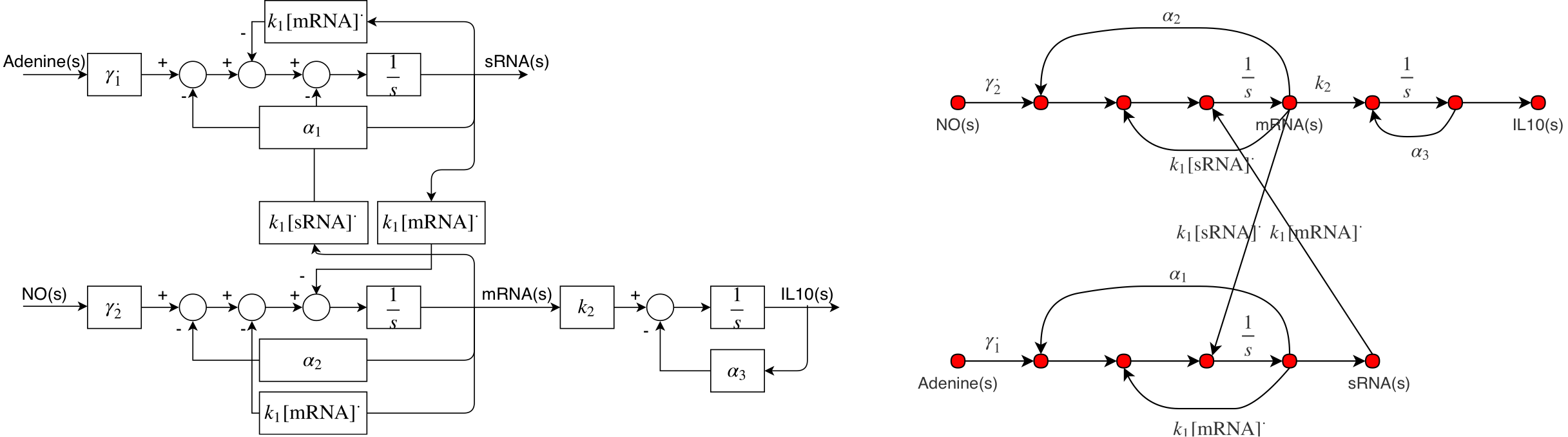
As stated in the assumptions, model has been linearised due to non-linearity raised by the Hill functions and sRNA binding; Hence, Hill functions have been replaced by \(\gamma_i^*\) -described below. The block diagram and signal flow graph for the linearised system are shown in Figure 2 , where transcription of IL10 mRNA, sRNA and translation of IL10 could be seen clearly.
$$ \gamma_i^* = \beta_i \frac{n_iK_i^{n_i}[u_i]^{n_i-1}}{(K_i^{n_i}+u_i^{n_i})^2} $$
Transfer functions for both negative and positive pathway were found using Mason's gain relation (Bolton &Newnes, 1998) and were double checked against(Steel &Papachristodoulou, 2017) . Transfer functions of both positive and negative pathways could be found below.
$$ G_1(s) = \frac{\text{IL10(s)}}{\text{Adenine(s)}} = \frac{k_2\gamma_1^*(s+\alpha_1+k_1[\text{IL10 mRNA}]^*)}{(s+\alpha_3)(s+s_+)(s+s_-)}, $$ $$ G_2(s) = \frac{\text{IL10(s)}}{NO(s)} = \frac{-k_1[\text{IL10 mRNA}]^*k_2\gamma_2^*}{(s+\alpha_3)(s+s_+)(s+s_-)}, $$
$$s_\pm = \frac{1}{2}(\alpha_2 + k_1[\text{sRNA}]^* + \alpha_1 +k_1[\text{IL10 mRNA}]^*)\pm \frac{1}{2}\sqrt{d},$$ $$d = (\alpha_2 + k_1[\text{sRNA}]^*- \alpha_1-k_1[\text{IL10 mRNA}]^*)^2+4k_1^2[\text{IL10 mRNA}]^*[\text{sRNA}]^*$$
Body response transfer function
Laplace transformed could be taken from both sides of the Equation [label] and by ignoring \(c\), being very small and negligible, we would be able to derive the transfer function for the body as shown below.
$$ s[\text{NO,Adenine(s)}] = -a_i[\text{NO,Adenine(s)}]+b_i[\text{IL10(s)}] \implies F_i(s) =\frac{[\text{NO,Adenine(s)}]}{[\text{IL10(s)}]} = \frac{b_i}{s+a_i} $$
Stability
The closed loop transfer function for cascade cascade controller design given in Figure 1 would contain importantinformation regarding steady state error and relative stability. It should be mentioned that similar to most control problems where the controller is designed for specific specifications (Dorf & H.Bishop, 1998), our reaction pathway could also be changed by changing promoter strength and length of sRNA, making it almost possible to adopt desired structures for the controller. The closed loop transfer function forpositive and negative pathways is as follow.
$$ T_i(s) = \frac{F_i(s)G_i(s)}{1+F_i(s)G_i(s)} $$
Based on the equation above, the stability of the system could be found by looking at the location of the poles which are the roots to the characteristic polynomial \(1+Fi(s)Gi(s)=0\). The characteristic equation was solved numerically and smallest poles and zeros for both reaction pathways are summarised in the Argand diagram below, Figure 3. All poles and Zeros are summarised after the figure. It should be noted that some poles and zeros were omitted as they were significantly larger than those shown in Figure 3 and would have thus hindered comparison with those illustrated. All poles and zeros are given below.
As stated earlier, not all poles have been plotted in the figure below as some are much larger in magnitude. Poles and Zeros for both responses are summarised in the table below.
| NO Response Poles | \(-1.075 \times 10^{4} \) | \(-0.030\) | \(-0.030\) | \(-1.060 \times 10^{-4}\) |
| NO Response Zeros | \(1.075 \times 10^{4} \) | \(-0.030\) | \(-0.030\) | \(-1.000 \times 10^{-4}\) |
| Adenine response Poles | \(-50.656\) | \(-0.474\) | \(-0.474\) | \(-0.262\) |
| Adenine response Zeros | \(-50.656\) | \(-50.000\) | \(-0.656\) | \(-1.000 \times 10^{-4}\) |
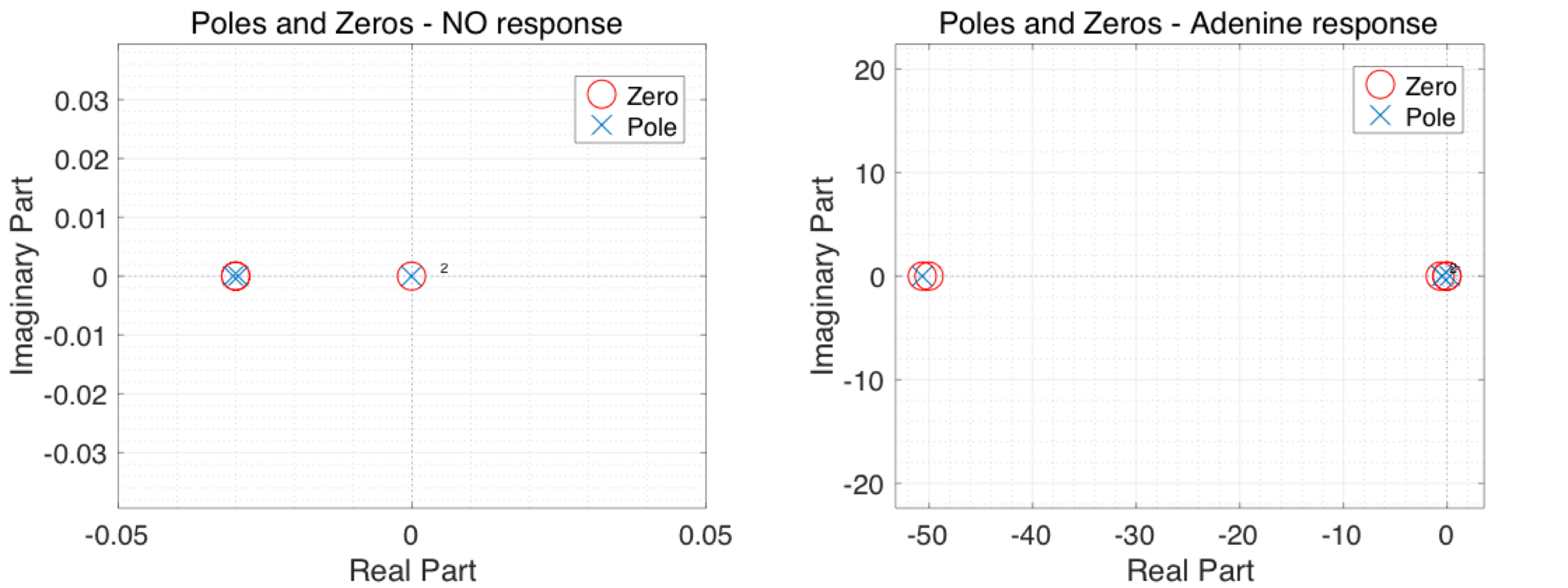
It could clearly be seen from the table and figure that all poles are real and negative which means the response of the system would be stabe and the transient part of the response will always decay exponentially without any oscillation or uncontrolled growth. This conclusion is crucial for our engineered E.coli as this would mean the combined model of body and E.coli would interact in a controlled way rather than a chaotic uncontrolled manner. Hence, the only remaining worry one might have would be the steady state error as the model tries to reach the healthy concentration of IL10. This issue is addressed later on the page.
DC Gain and Steady State Error
The steady state error could be easily found using the cascade compensation model demonstrated earlier and the Final value Theorem(FVT). The steady state error would be \( \lim_{t\rightarrow \infty} e(t) \) which coupled to FVT could be written as \(\lim_{s \rightarrow 0} sE(s)\), where \(E(s)\) is the Laplace transform of the error. \(E(s)\) could be written as follow.
$$ E(s) = \frac{1}{1+G_i(s)F_i(s)}R(s) \; , \; R(s) = \frac{C}{s} \quad C \in \mathbb{R} $$ $$FVT \, :\quad \lim_{t\rightarrow \infty} e(t) = \lim_{s \rightarrow 0} sE(s)$$ $$\therefore \; \lim_{t \rightarrow \infty} e(t) = \lim_{s\rightarrow 0} \frac{1}{1+G_i(s)F_i(s)} $$By substituting back Transfer functions for both E. Coli,\(G_i(s)\), and the body,\(F_i(s)\), the steady state error can be found as follows:
- For NO response \(\lim_{t\rightarrow\infty} e(t) =-2.9501\times10^{-4} \).
- For adenine response \(\lim_{t\rightarrow\infty} e(t) = -2.1912\times10^{-3} \).
It is evident that the combined model has a very small DC gain and hence, a very small margin of error is estimated for the steady concentration of IL-10.