Team:Queens Canada/Fluid Dynamics

Fluid Dynamics

Obtaining a Sufficient Amount of Saliva

Known variables from QGEM resources and equations from literature are employed to characterize the fluid dynamics of the pacifier. The protein size is given at 77 kilodaltons, with a concentration in water (as a protein solution) of 2.37 mg/ml. Based on previous work, it can be assumed that an infant is able to product a mean value of 4μL per second of saliva [1][2]. For adequate interaction of saliva with the protein solution 100μL of saliva is required to accumulate within the well. Using the diameter of 1.5mm and length of 12mm for the saliva channel connecting the nipple to the pacifier internals the total required volume of saliva required was calculated to be 184.78μL as shown.

V_required = V_tube + 100μL
V_required = π(0.0015m)²(0.012m) + 100μL
V_required = 184.23μL

This volume of saliva could theoretically be produced by an infant in under 60 seconds. However, it should be noted that actual saliva collection rates may be lower than those found in literatures as those reported values were associated with syringe extraction from the lip of the patient, while QGEM’s pacifier uses a more passive collection mechanism. Even with extraction rates five time lower than found in literature, the collection process would take place in less than five minutes which is reasonable and achievable for a typical collection period. Further research should be conducted to determine the flow rate of saliva using QGEM’s pacifier mechanism.

Characterizing saliva flow

Reynolds Number

In order to analyze the flow of the saliva using Reynolds number, the dynamic viscosity and density of saliva are needed. Following a literature review’s, a mean value of 0.0023 Pa∙s, was determined to be the dynamic viscosity of human saliva [3][4], with a mean density of 978 kg∙m-3 [5]. Additionally, to determine the exact Reynolds number a fluid velocity is required, or a desired Reynolds number may be assigned to calculate the necessary velocity.

The Reynolds number equation is shown below where ρ is the density of the fluid (kg∙m-3), D is the diameter (m), V is the velocity of the fluid (m∙s-1), and μ is the dynamic viscosity of the fluid (Pa∙s).

Re = ρDV/μ

From the calculation of the Reynolds number, all salivary flow within the pacifier corresponds to laminar flow (Re <2100). This calculation holds at speeds of up to 1000 m/s, while actual fluid speeds within the pacifier will be in the order of magnitude of centimetres per second. Stokes flow, or creeping flow, is also applicable to this situation, since the Reynolds number is extremely small (around 10-6, where Stokes flow is Re << 1). This indicates that flow within the pacifier will take on a parabolic flow profile as shown below.

Surface Tension

To ensure that flow is possible in the desired direction the contact angle between the channel and saliva must be considered. The contact angle quantifies the wettability of a solid surface through its liquid, vapour, solid phase interactions. The degree of wetting indicates the ability for a liquid surface to maintain contact with a solid as determined by a force balance between the adhesive of the solid and liquid that force the liquid to spread, and the cohesive forces that hold the liquid together.

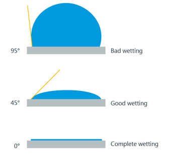
To ensure that flow is possible in the desired direction we must use a solid surface that interacts with the liquid more strongly than the saliva does with itself to achieve good wetting. A hydrophilic surface will ensure that the contact angle is less than 90 degree’s and therefore allow fluid flow. Silicone's are naturally hydrophobic, such that a surfactant will be required to reduce the surface tension at the liquid solid interface and thus increase wetting.

Pressure Needed to Translate Saliva

External Driving Force

The Navier-Stokes equations can be used in this simple pipe flow model to determine the differential pressure, since it is assumed that the saliva flow is laminar, has a constant density, and is Newtonian [6].

With the further assumptions of a fully developed, steady, axisymmetric, and no radial component flow the Navier Stokes Equation can be simplified to the Hagen-Poiseulle equation. The Hagen-Poiseuille equation is shown below, where ∆P is the pressure drop across the two pipe ends (Pa), μ is the dynamic viscosity of the fluid (Pa∙s), L is the length of the pipe (m), Q is the volumetric flow rate of the fluid (m3∙s-1), and R is the radius of the pipe (m).

ΔP = 8μLQ/πR⁴

Rearranging the Hagen-Poiseuille equation shows that the flow rate is proportional to the pressure drop and radius, and inversely proportional to the viscosity and pipe length. The pressure drop along the tube using the variables previously identified is shown below.

ΔP = 8 * 0.0023Pa⋅s * 0.012m * 4⋅10^-9⋅s^-1/π⋅(0.00075m)⁴
ΔP = 0.8885Pa

A small pressure drop of 0.8885 Pa could easily be overcome by use of an external pressure creating device (ie. nasal respirator) or by tilting the pacifier during saliva collection using gravitational energy to transport the saliva from the inner tubing to the protein chamber.

Bond Number

The Bond number can be used to further characterize the driving force of fluid as a comparison of the importance of gravitational forces to surface tension force. To calculate the Bond number, the surface tension of saliva, and density of plastic tubing are required along with the variables previously identified. Following a literature review, a mean value of 0.0589 N/m was determined to be the surface tension of saliva [7], and the density of 1100-2300 kg∙m-3 was used for a range of silicon plastics [8].

The Bond number (Bo) equation is shown below where Δρ is the density difference of the fluid and plastic (kg∙m-3), g is the gravitational constant (m/s2), D is the diameter of the tubing (m), and σ is the surface tension of the saliva (N/m).

Bo = Δρ⋅g⋅D²/σ

The bond number for the pacifier was calculated as shown below for the high and low plastic density range.

Bo = (2300-978)kg⋅m^-3⋅9.8m⋅s^-2⋅(0.0015m)²/0.0589N⋅m^-1
Bo = 329.94

Bo = (1100-978)kg⋅m^-3⋅9.8m⋅s^-2⋅(0.0015m)²/0.0589N⋅m^-1
Bo = 30.44

Using a high-density plastic, resulting in a high bond number indicates that the system is relatively unaffected by surface tension, whereas the low-density plastic resulting in an intermediate bond number indicates a trivial balance between the two forces. For surface tension to be the dominant force, a bond number less than one would be required however this is not a realistic based on potential tubing materials. Alternatively, the diameter of the tubing can be reduced such that surface tension becomes the dominant force for a chosen plastic.

Capillary Action

To further explore the effect of surface tension as a driving force for fluid flow, the Young-Laplace equation can be used to determine the height of capillary action based on the wettability of the surface. The Young-Laplace equation is shown below, where ΔP is the pressure drop that can be overcome by capillary action, σ is the surface tension of the saliva (N/m), θ is he contact angle between the saliva and tubing, and R is the radius of the tube (m).

ΔP = 2⋅σ⋅cosθ/R

For a sufficiently narrow tube (ie. Low bond number) the induced capillary pressure is balanced by the change in height, which will be positive for wetting angles less than 90˚. The height achieved at this hydrostatic equilibrium can be calculated by rearranging the Young-Laplace equation and setting it equal to the gravitational forces, as shown below.

h = 2⋅σ⋅cosθ/ρ⋅g⋅R

Using tube surface that is just hydrophilic with a wetting angle of 89˚ the height achieved by capillary action is shown below.

h = 2⋅0.0589N⋅m^-1⋅cos(89)/978kg⋅m^-3⋅9.8m⋅s^-2⋅0.00075m
h = 0.268mm

Evidently, for capillary action to significantly impact the driving force of the moving the saliva, a very hydrophilic surface must be used. The contact angle necessary to propel the saliva over the length of 12mm can be calculated by rearranging the above equation.

θ = cos^-1(ρ⋅g⋅R⋅h/2⋅σ)
θ = cos^-1(978kg⋅m^-3⋅9.8m⋅s^-2⋅0.00075m⋅0.012m/2⋅0.0589N⋅m^-1)
θ = 42.9°

To achieve this wetting angle, various surfactants can be used to increase the wettability of the surface [10] [11].

Brownian Model of Saliva in Protein Solution

As a theoretical model for the project, the team decided to examine the Narrow Escape problem as it pertains to particles in a 96-well plate. The Narrow Escape problem is a famous problem in Brownian motion, or simply the motion of particles in a solution; given a container with an opening and a particle placed inside, what is the average time for the particle to escape from the container if the particle is moving randomly?

The solution to this problem depends on many variables, including the particle, the size of the container and the size of the opening. For the purposes of this experiment, 96 well plates were used as the container. The aim was to determine if the narrow escape time for a particle produced during a biochemical reaction would change depending on the shape of the 96 well plates. A container with a shorter narrow escape time would have the particle leaving the container in the fastest time, which would be desirable in many situations. As such, the various shapes of the 96-well plates were tested to see which would produce the shortest time.

The tests were run using MATLAB software. First, a model of the given container was created. Then, a particle was placed randomly in the container, and subjected to simple random walk motion. After the particle was noted to have left the container the amount of time was recorded, and the trial was repeated.

Known variables from QGEM resources and equations from literature are employed to characterize the fluid dynamics of the pacifier. The protein size is given at 77 kilodaltons, with a concentration in water (as a protein solution) of 2.37 mg/ml.

The motion of cortisol within saliva has been modelled with MATLAB, as shown below. The motion of cortisol within saliva mixing with the protein solution is also valuable to model. This allows for the quantification of light-producing reactions between cortisol and the protein. Unfortunately, an error found within the MATLAB code was never fully solved, which limited the effectiveness of calculations performed using this model. Further mathematical modelling is included in another section. The MATLAB code can be found here:

Brownian model in MATLAB

anArray = zeros(1,10);          %Initialize storage array
storageCounterMax = 10;

for storageCounter = 1:storageCounterMax

%Variable Declaration
n = 1;                          %Initialize loop counter
N=0.25;                         %Range from random selection will be [-N,N]
loopMax=10000;                  %Number of random walk movements
ColorSet = varycolor(loopMax);  %Set amount of colours
diameter = 6.94;                %Set diameter of cylinder
radius = diameter*0.5;          %Set radius of cylinder
totalHeight = 10.85;            %Set total height of container
pauseTime = 0.0;                %Set time between plotting iterations
boundaryCondition = true;

%Cylinder Figure
maxHeight = totalHeight - radius;
h=maxHeight;
x0=0;y0=0;z0=0;
[x,y,z]=cylinder(radius);
x=x+x0;
y=y+y0;
z=z*h+z0;

%Half Sphere Figure
A = [0 0 0 radius];
[X, Y, Z] = sphere;
XX = X * A(4) + A(1);
YY = Y * A(4) + A(2);
ZZ = Z * A(4) + A(3);
XX = XX(11:end,:);
YY = YY(11:end,:);
ZZ = -ZZ(11:end,:);

%Display Information
figure
xlabel('X');
ylabel('Y');
zlabel('Z');
surface(x,y,z, 'FaceAlpha', 0.1, 'FaceColor', [ 1 1 0], 'EdgeColor', [0.4, 0.4, 0.4]); hold on
surface(XX, YY, ZZ, 'FaceAlpha', 0.1, 'FaceColor', [ 1 1 0], 'EdgeColor', [0.4, 0.4, 0.4]); hold on
axis equal
view(3);
set(gca,'GridLineStyle','-')
Information=strcat('Brownian Motion in 3D Space');
title(Information ,'FontWeight','bold');
view(-109,40);
hold all
set(gca, 'ColorOrder', ColorSet);


%Initialize Beginning Location
heightInitialize = maxHeight + radius;
xF = (2*radius*rand())-radius;
yF = (2*radius*rand())-radius;
zF = (heightInitialize*rand())-radius;

while(boundaryCondition == true)
    
    n = n + 1;

    xI = xF;
    yI = yF;
    zI = zF;

    xF = xI + (2*N*rand())-N;
    yF = yI + (2*N*rand())-N;
    zF = zI + (2*N*rand())-N;
    
    dist = sqrt(xF^2 + yF^2);
    length = sqrt(xF^2 + yF^2 + zF^2);

    
    if (zF >= maxHeight)
        flag = 1;
        disp(n);
        break;
    end
    
    if (zF >= 0 && zF < maxHeight && dist < radius)

        v1=[xI,yI,zI];
        v2=[xF,yF,zF];
        v=[v2;v1];
        plot3(v(:,1),v(:,2),v(:,3));
        pause(pauseTime);
    
    elseif (zF < 0 && length < radius)
        
        v1=[xI,yI,zI];
        v2=[xF,yF,zF];
        v=[v2;v1];
        plot3(v(:,1),v(:,2),v(:,3));
        pause(pauseTime);
    
    else
        
        boundaryCondition = false;
        while(boundaryCondition == false)
       
            xF = xI + (2*N*rand())-N;
            yF = yI + (2*N*rand())-N;
            zF = zI + (2*N*rand())-N;

            length = sqrt(xF^2 + yF^2 + zF^2);
            dist = sqrt(xF^2 + yF^2);
        
            if ((zF >= 0 && zF < maxHeight && dist < radius)||(zF < 0 && length < radius))
                boundaryCondition = true;
                v1=[xI,yI,zI];
                v2=[xF,yF,zF];
                v=[v2;v1];
                plot3(v(:,1),v(:,2),v(:,3));
                pause(pauseTime);
                
            end
        end
    end
end

anArray(storageCounter)=n;
disp(anArray);
end

plot3(xF,yF,zF,'ok','MarkerFaceColor','r');
hold off
disp(anArray)
disp(n)

function ColorSet=varycolor(NumberOfPlots)
% VARYCOLOR Produces colors with maximum variation on plots with multiple
% lines.
%
%     VARYCOLOR(X) returns a matrix of dimension X by 3.  The matrix may be
%     used in conjunction with the plot command option 'color' to vary the
%     color of lines.  
%
%     Yellow and White colors were not used because of their poor
%     translation to presentations.
% 
%     Example Usage:
%         NumberOfPlots=50;
%
%         ColorSet=varycolor(NumberOfPlots);
% 
%         figure
%         hold on;
% 
%         for m=1:NumberOfPlots
%             plot(ones(20,1)*m,'Color',ColorSet(m,:))
%         end

%Created by Daniel Helmick 8/12/2008

narginchk(1,1)%correct number of input arguements??
nargoutchk(0, 1)%correct number of output arguements??

%Take care of the anomolies
if NumberOfPlots<1
    ColorSet=[];
elseif NumberOfPlots==1
    ColorSet=[0 1 0];
elseif NumberOfPlots==2
    ColorSet=[0 1 0; 0 1 1];
elseif NumberOfPlots==3
    ColorSet=[0 1 0; 0 1 1; 0 0 1];
elseif NumberOfPlots==4
    ColorSet=[0 1 0; 0 1 1; 0 0 1; 1 0 1];
elseif NumberOfPlots==5
    ColorSet=[0 1 0; 0 1 1; 0 0 1; 1 0 1; 1 0 0];
elseif NumberOfPlots==6
    ColorSet=[0 1 0; 0 1 1; 0 0 1; 1 0 1; 1 0 0; 0 0 0];
    
else %default and where this function has an actual advantage

    %we have 5 segments to distribute the plots
    EachSec=floor(NumberOfPlots/5); 
    
    %how many extra lines are there? 
    ExtraPlots=mod(NumberOfPlots,5); 
    
    %initialize our vector
    ColorSet=zeros(NumberOfPlots,3);
    
    %This is to deal with the extra plots that do not fit nicely into the
    %segments
    Adjust=zeros(1,5);
    for m=1:ExtraPlots
        Adjust(m)=1;
    end
    
    SecOne   =EachSec+Adjust(1);
    SecTwo   =EachSec+Adjust(2);
    SecThree =EachSec+Adjust(3);
    SecFour  =EachSec+Adjust(4);
    SecFive  =EachSec;

    for m=1:SecOne
        ColorSet(m,:)=[0 1 (m-1)/(SecOne-1)];
    end

    for m=1:SecTwo
        ColorSet(m+SecOne,:)=[0 (SecTwo-m)/(SecTwo) 1];
    end
    
    for m=1:SecThree
        ColorSet(m+SecOne+SecTwo,:)=[(m)/(SecThree) 0 1];
    end
    
    for m=1:SecFour
        ColorSet(m+SecOne+SecTwo+SecThree,:)=[1 0 (SecFour-m)/(SecFour)];
    end

    for m=1:SecFive
        ColorSet(m+SecOne+SecTwo+SecThree+SecFour,:)=[(SecFive-m)/(SecFive) 0 0];
    end
end
end

Diagram showing Brownian simulations in a tube

References

[1] C. J. Bacon, J. C. Mucklow, A. Saunders, M. D. Rawlins, and J. K. Webb, “A method for obtaining saliva samples from infants and young children.,” Br. J. Clin. Pharmacol., vol. 5, no. 1, pp. 89–90, Jan. 1978.
[2] “Saliva Collection from Infants and Small Children,” 02-Jun-2017. [Online]. Available: https://www.salimetrics.com/saliva-collection-from-infants-and-small-children/. [Accessed: 29-Jul-2018].
[3] E. Sajewicz, “Effect of saliva viscosity on tribological behaviour of tooth enamel,” Tribol. Int., vol. 42, no. 2, pp. 327–332, 2009.
[4] M. Negoro et al., “Oral glucose retention, saliva viscosity and flow rate in 5-year-old children,” Arch. Oral Biol., vol. 45, no. 11, pp. 1005–1011, 2000.
[5] P. J. Lamey and A. Nolan, “The recovery of human saliva using the Salivette system,” Eur. J. Clin. Chem. Clin. Biochem. J. Forum Eur. Clin. Chem. Soc., vol. 32, no. 9, pp. 727–728, Sep. 1994.
[6] Noel de Nevers, “Fluid Mechanics for Chemical Engineers,” 2nd ed., McGraw-Hill, Inc., 1991, pp. 275–279.
[7] Lam, J C M et al. “Saliva Production and Surface Tension: Influences on Patency of the Passive Upper Airway.” The Journal of Physiology 586.Pt 22 (2008): 5537–5547. PMC. Web. 12 Oct. 2018.
Silicone
[8] “Properties: Silicone Rubber.” AZoM.com, www.azom.com/properties.aspx?ArticleID=920.
[9] A. A. Abdul-Hadi and A. A. Khadom, “Studying the Effect of Some Surfactants on Drag Reduction of Crude Oil Flow,” Chinese Journal of Engineering, 2013. [Online]. Available: https://www.hindawi.com/journals/cje/2013/321908/. [Accessed: 04-Aug-2018].
[10] S. Lyu, D. C. Nguyen, D. Kim, W. Hwang, and B. Yoon, “Experimental drag reduction study of super-hydrophobic surface with dual-scale structures,” Appl. Surf. Sci., vol. 286, pp. 206–211, Dec. 2013.
[11] P. Argyrakis and R. Kopelman, “Self-stirred vs. well-stirred reaction kinetics,” J. Phys. Chem., vol. 91, no. 11, pp. 2699–2701, May 1987.