Team:SKLMT-China/Model Process
Background
We have built a promoter library of inner promoters with various strength in
1.To facilitate the promoter transformation of pseudomonas fluorescence in new site;
2.To reveal the correlation between promoter weights and their strength;
4.To improve the parameter setting of the promoter strength prediction in the species outside the large intestine with the method of position weight;
5.To provide reference for other microbe promoter strength prediction modeling.
Assumptions
1. It is assumed that the promoter strength is only related to the core DNA sequence.In other words, the DNA sequence can uniquely determine the promoter strength.
2. It is assumed that the laboratory environment has no impact on the test results.In other words, our test data can fully reflect the promoter strength.
3.It is assumed that there is a simple monotonic relationship between the obtained fluorescence data and the promoter strength: the larger the fluorescence value is, the stronger the promoter can be considered.
Modelling Process
DNA Sequence Encoding
The 5’-3’ region includes 70bp DNA information in each promoter. Currently, we have got 25 promoter sequences. We need to encode these 70 bases in order to establish a mathematical model. Notice that there’re only four types of bases(A,T,C and G),and calculating the numbers of each type is not enough to reflect interaction between adjacent bases.[2] Thus, we consider 3 continuous bases
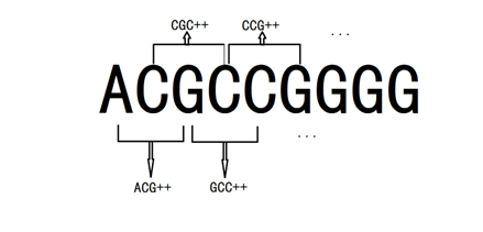
We encode each three-base sequence with quaternary number(A,T,C,G represents quaternary number 0,1,2,3 ), and by running a C++ program (the whole code is shown in appendix), we get a vector with 64 dimensions from AAA to GGG, which calculates the frequency of appearance for each type in DNA sequence.
After encoding, all DNA sequences are transformed into a vector with 64 dimensions. The entire data is stored in the document
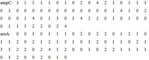
At the end of the encoding step, we get an 25*64 matrix which reflects the features of these DNA sequences of each promoters. This encoding method has deep internal connection with the characteristics of DNA sequence, and it simultaneously contains the sequential relationship and details of DNA sequence. With this matrix, a mathematical model can be established.
Model establishment and solution
In order to simplify the problem, we assume that the connect between matrix and promoter strength is linear, in other words, the vector \({x}\) exists when equation \({y=Ax}\) is satisfied.
Now, through a lot of experiments, we have measured a total of 24 values, and all twenty-two valid values are shown below. Each data is the average of the results of three parallel experiments.
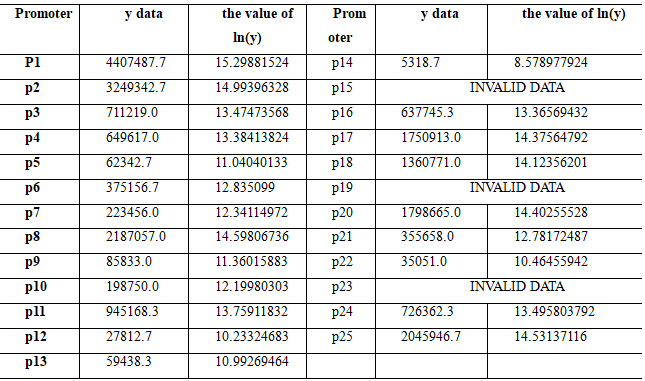
The gap in original data is too wide, so we take the natural log of the original data as the value of the vector . Now, what we're going to do is to invert the linear relationship vector \({x}\) by taking the linear transformation matrix \({A}\) and the resulting vector \({y}\).\({A,x}\) and \({y}\)satisfy the following equation: \({y=Ax}\),or \({x=A^{-1}y}\).
This is a linear mapping of 64 variables but there are only 22 data points. In other words, this is an underdetermined equation which cannot be solved accurately by solving inhomogeneous linear equations. The sparse solution algorithm of underdetermined equations based on iteration3 will be adopted in the following part.
This is an effective algorithm to restore deterministic signals with fewer premeasured values.Our goal is to improve the precision of signal reduction as much as possible. Consider the following optimization problem:
$$min \left \| x \right \|_{0}$$ $$s.t.\; \; \; y=Ax$$\(\left \| x \right \|_{0}\)is called \(l^{0}\)norm, which represents the number of nonzero components in vector x in mathematics. This value is equivalent to this expression:
$$\lim_{\varepsilon \rightarrow 0}\sum_{i=1}^{64}\frac{x_{i}^{2}}{x_{i}^{2}+\varepsilon }, because\frac{x_{i}^{2}}{x_{i}^{2}+\varepsilon }= \begin{cases} & \text{ 0, } x_{i}=0 \\ & \text{ 1, } x_{i}\neq 0 \end{cases} (\varepsilon \rightarrow 0)$$The following iterative steps are obtained from the perspective of numerical calculation:
⑴At first , set the initial \({x^{(0)}=0}\),\({\varepsilon ^{(0)}=1}\)value
⑵After that, loop to calculate the current \({x^{(n+1)} }\),\({\varepsilon ^{(n+1)}}\)value based on the previous value \({x^{(n+1)} }\),\({\varepsilon ^{(n+1)}}\) with this formula:
$$x^{(n+1)}=arg\, min\left \{ \sum_{i=1}^{64}\frac{x_{i}^{2}}{(x_{i}^{(n)})^{2}+\varepsilon^{(0)} } \right\},(y=Ax);$$ $$\varepsilon ^{(0)}=min\left \{ \varepsilon ^{(n)} ,\frac{min(x_{i}^{(n)})}{N}\right \}$$⑶Finally, if is less than a given bound such as 1e-6, abort this program, and regard current \({x^{(n)}}\) as the solution vector of this underdetermined equation.
The explicit iterative form of the above steps is given below:
$$ f(x,\lambda )=\sum_{i=1}^{64}\frac{x_{i}^{2}}{{(}x_{i}^{(n)})^{2}+\varepsilon ^{(n)}}=\sum_{i=1}^{64}\frac{x_{i}^{2}}{{(}x_{i}^{(n)})^{2}+\varepsilon ^{(n)}}+\lambda (Ax-y)$$we use Lagrange multiplier method to solve the minimum variable. Vector \({\lambda }\)with 22 dimensions is introduced. So calculate the partial derivative to each component of \({x}\),then solve this equation:
$$\frac{\partial f}{\partial x_{i}}=0$$We find that the vector \({x}\)can be iterated by this formula:
$$x^{(n+1)}=D^{(n)}{A}'(AD^{(n)}{A}')^{-1}y.$$where we construct matrix \({D^{(n)} }\) as follow:
$$D^{(n)}_{ij}= \begin{cases} & \text{ 0, } i\neq j \\ & \text (x_{i}^{(n)})^{2}+\varepsilon ^{n},i=j \end{cases}$$With the help of
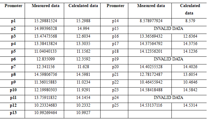
Part of the value without bold is used to solve the equation, so it is a perfect match; From the comparison of data in bold, it can be seen that the result of data fitting is good, with the average fitting degree higher than 95%.
The solution results of the matrix are good, which confirms the basic reliability of the assumed linear relationship. Therefore, we will use the neural network model to further improve the accuracy and stability of the model prediction.
Model Improvement--Algorithm optimization
By solving the matrix sparse solution algorithm, we can conclude that there is indeed a linear relationship between the total 64 data of AAA-GGG and the promoter strength. Notice that we used merely 22 sets of data to approximately solve the sparse solutions of 64 equations with a fitting precision higher than 95%, therefore, when we provide as much data as possible, the fitting precision of the model will greatly increase.
However, there are still many problems with this algorithm:
(1) All known data cannot be reused. The sparse solution is uniquely calculated as the data is determined, so the data is not very well utilized, and it is difficult to improve the accuracy of the original results as well.
(2) This algorithm is not well adapted to the extension of existing data sets. Every time a new set of data is added, all matrix operations change apparently, so it's not very stable when data updates.
On the basis of the linear structure of the original algorithm, we add more parameters to make the algorithm more stable and reliable. This algorithm adopts the neural network structure and improves the utilization rate of data by supervised learning.The construction of neural network is shown in the Figure 2:
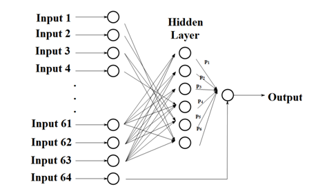
There are 6 neurons in the hidden layer, and each neuron is connected with 32 input terminals. The corresponding relation is as follows: The binary number of integer 1~63 is exactly 6 bits, and the deficiency is added. Input and hidden neuron \({j}\)is connected when the \({ j^{th}}\) number of the binary number is 1. In particular, we consider port 64 separately.And then we give a certain weight \({\omega _{ij}}\) to each edge between Input \({i}\)and hidden neuron \({j}\),and give to each edge between hidden neuron \({ p^{i}}\)and output terminal.
The final output can be obtained by the following formula:
$$y_{output}=\sum_{i=1}^{6}y_{i}p_{i},y_{i}=\sum_{j=1}^{64}\omega _{ji}x_{j}\, \; .$$\({y_{i}}\)represents the input(output) data of hidden neuron \({i}\).
We use gradient descent method to determine the learning direction. The objective function is the error of output and ideal values:
$$e=\frac{1}{2}(y_{output}-\bar{y})^{2}$$Our goal is to minimize the value of this function by generations of iterations. Difference between vector , \({ \omega =(\omega _{16},...,\omega _{n6})}\),\({p=(p_{1},...,p_{n}) }\)and its next generation is calculated by this formula:
$$y_{output}=\sum_{i=1}^{6}y_{i}•p_{i},y_{i}=\sum_{j=1}^{64}\omega _{ji}x_{j}.$$\({y_{i}}\)represents the input(output) data of hidden neuron \({i}\).
We use gradient descent method to determine the learning direction. The objective function is the error of output and ideal values:
$$e=\frac{1}{2}(y_{output}-\bar{y})^{2}$$Our goal is to minimize the value of this function by generations of iterations. Difference between vector , \omega =(\omega _{16},...,\omega _{n6}),p=(p_{1},...,p_{n}) and its next generation is calculated by this formula:
$$ \Delta \omega =-v\cdot grad\omega ,\Delta p=-v\cdot gradp$$where \({v}\)represents learning speed. We use the chain rule to calculate the specific value of the gradient:
$$\begin{cases} & \text{ if } \frac{\partial e}{\partial \omega_{ij} }= (y_{output}-\bar{y})\frac{\partial y_{output}}{\partial \omega _{ij}}=(y_{output}-\bar{y})x_{i}p_{j}\\ & \text{ if } \frac{\partial e}{\partial p_{i}}= (y_{output}-\bar{y})\frac{\partial y_{output}}{\partial p_{i}}=(y_{output}-\bar{y})y_{i} \end{cases}$$At the same time, a reasonable learning speed is designed for the program, which can accelerate the convergence speed while ensuring the convergence. After several convergence tests, we set the learning speed as\({0.00045\cdot \left | y_{output}-\bar{y} \right |.}\)That's where our mathematical model comes in.
Model analysis and evaluation
After improvement of the above algorithm, the advantages of the model are as follows:
1. High stability of the model. This algorithm adopts the mode of deep learning, which shortens the step length of vector change and expands the relevant linear parameters to 206, ensuring the precision of model fitting and greatly improving the stability of the model.
2. The input of the model can be extended conveniently. When the data of the promoter library is expanded, it only needs to input the latest measured data into our system, which is automatically imported into the database, and the model can also use this data for training immediately.
3. The method of this model can be used for reference by other subjects. The coding method and mathematical treatment of the model are in line with the effect of DNA sequence on the promoter strength and can be transplanted to other similar studies such as
At the same time, there are also many deficiencies in this model that need to be improved:
1. The model is not robust to error data. When a group of incorrect fluorescent values are given in the input data, the fitting precision of the whole program will be greatly affected, and this interference will gradually weaken as the number of correct data increases.
2. Convergence speed and accuracy still need to be improved. If the number of training rounds is too high, the running speed of the program is too slow. When the number of rounds is too low, the results presented are often unsatisfactory. We need to find a balance between speed and accuracy.
References
[1]Lim, C. K.Hassan, K. A.Tetu, S. G.Loper, J. E.Paulsen, I. T. The effect of iron limitation on the transcriptome and proteome of Pseudomonas fluorescens Pf-5. PLoS One. 2012, June 2012 | Volume 7 | Issue 6 | e39139,2-18
[2] Xuan Zhou, Xin Zhou, Zhaojie Zhong, Prediction of start-up strength of E. coli promoter, Computers and Applied Chemistry, Jan.28,2014|Volume 31| Issue 1,101-103
[3]Xiaoliang Cheng, Xuan Zheng, Weimin Han, An algorithm for solving sparse solutions of undetermined linear equations,College journal of applied mathematics,2013:28(2):235-248