Team:UESTC-China/Model butanol

team

1. Introduction

We hope to obtain the yield function of butanol using experimental data. The optimal fermentation conditions and maximum yield were obtained for the optimal solution of the function. Then we tried again under the best fermentation conditions. The result shows that the yield has obviously increased.

The molecular dynamics model has been established, and the speed limiting steps and the parameters with high sensitivity have been found. The efficiency of the system can be further improved by optimizing the speed limiting steps of the reaction and the parameters with high sensitivity.
2. Optimization of butanol fermentation process

Increasing the yield and rate of butanol is a hot and difficult point in current biobutanol research. Butanol synthesis is affected by many environmental conditions such as temperature, inoculum (initial OD), and initial pH. We constructed a kinetic equation for the synthesis of butanol, and optimized the butanol synthesis condictions to increase butanol production [1].

2.1 Experiment design

In the butanol fermentation process, how to control the temperature (\({x_1}\)),initial OD (\({x_2}\)), initial pH (\({x_3}\)), so that is the butanol yield (\(y\)) the highest? To do this, we need to explore the quantitative relationship between y and \({x_1}\), \({x_2}\), \({x_3}\). The quantitative relationship between them can be expressed by the following model:

\[y = f({x_1},{x_2},{x_3})\]

Since the response surface equation \(y = f({x_1},{x_2},{x_3})\) is unknown , a test (sampling) is required, and the experimental data obtained from the finite test is used to estimate \(f\) (by partial estimation of the whole). We chose the Box-Behnken Design (BBD) method to design the experiment [2][3]. The test point arrangement is shown in Fig. 1.

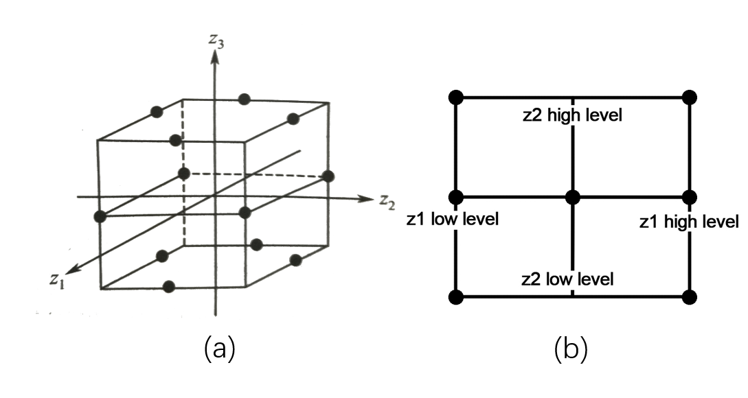Fig. 1 (a)test points for Box-Behnken design (b)test points projection on z1, z2 plane

The maximum and minimum values of \({x_1}\)，\({x_2}\)， \({x_3}\) are called upper levels and lower levels, and the average of upper levels and lower levels is zero levels. Since the dimensions of \({x_1}\)，\({x_2}\)，\({x_3}\) are different, you need to standardize the variables:

\[{z_i} = \frac{{{x_i} - \overline {{x_i}} }}{\sigma }\]

Where, \({z_i}\) is the normalized variable (encoding), \(\overline {{x_i}} \) is the average, and \(\sigma \) is the standard deviation. The variation range and normalized value of \({x_1}\)，\({x_2}\)， \({x_3}\) are as follows:

Table 1 Levels of the variables of Box–Behnken design

Code	Variable	Low level(-1)	Zero level(0)	High level(+1)
\[{x_1}\]	Temperature(℃)	31	34	37
\[{x_2}\]	Initial OD	11	16	20
\[{x_3}\]	Initial pH	6	7	8

2.2 Model establishment

The test points of the BBD test design and the corresponding experimental data are shown in the following table:

Table 2 The Box–Behnken experimental design with three independent variables

Test number	\[{z_1}\]	\[{z_2}\]	\[{z_3}\]	\(y\)(g/L)
1	0	0	0	0.246
2	0	0	0	0.247
3	0	0	0	0.246
4	0	1	1	0.333
5	0	1	-1	0.177
6	-1	0	1	0.206
7	1	-1	0	0.112
8	0	0	0	0.246
9	-1	-1	0	0.111
10	-1	1	0	0.258
11	1	0	-1	0.191
12	1	1	0	0.209
13	0	-1	1	0.279
14	0	-1	-1	0.161
15	-1	0	-1	0.183
16	0	0	0	0.245
17	1	0	1	0.211

Multivariate regression analysis of the experimental data was performed using Design-Expert11, and the following third-order polynomial equations were found to explain the generation of butanol:

\[\begin{array}{l} y = 0.2460 - 0.0032{z_1} + 0.0175{z_2} + 0.0685{z_3} - 0.0125{z_1}{z_2}\\ - 0.0008{z_1}{z_3} + 0.0095{z_2}{z_3} - 0.0566{z_1}^2 - 0.0169{z_2}^2 + 0.0084{z_3}^2\\ + 0.0435{z_1}^2{z_2} - 0.0578{z_1}^2{z_3} - 0.0152{z_1}{z_2}^2 \end{array}\]

(1)

The variance analysis of the regression analysis results is shown in the following table:

Table 3 ANOVA of regression equation of butanol yield

Source	Sum of Squares	\[df\]	Mean Square	F-value	P-value
Model	0.0522	12	0.0043	8698.31	< 0.0001
\[{z_1}\]	0	1	0	84.5	0.0008
\[{z_2}\]	0.0012	1	0.0012	2450	< 0.0001
\[{z_3}\]	0.0188	1	0.0188	37538	< 0.0001
\[{z_1}{z_2}\]	0.0006	1	0.0006	1250	< 0.0001
\[{z_1}{z_3}\]	0	1	0	4.5	0.1012
\[{z_2}{z_3}\]	0.0004	1	0.0004	722	< 0.0001
\[{z_1}^2\]	0.0135	1	0.0135	27001.18	< 0.0001
\[{z_2}^2\]	0.0012	1	0.0012	2398.03	< 0.0001
\[{z_3}^2\]	0.0003	1	0.0003	590.66	< 0.0001
\[{z_1}^2{z_2}\]	0.0038	1	0.0038	7569	< 0.0001
\[{z_1}^2{z_3}\]	0.0067	1	0.0067	13340.25	< 0.0001
\[{z_1}{z_2}^2\]	0.0005	1	0.0005	930.25	< 0.0001
Pure Error	0	4	0
Cor Total	0.0522	16
Coefficient of determination \[{R^2} = 0.9998\]			Adequate Precision=359.0217

The variance analysis of the regression analysis results is shown in the following table: the F-value is 8698.31 and the P-value <0.0001, indicating that the model fits well, and the model's goodness of fit \({R^2}\) is 0.9998, indicating that the regression model 99.98% explains the response. Only 0.02% of the model's changes cannot be explained by the model. Moreover, accuracy is used to describe the signal-to-noise ratio of the model [4]. The signal-to-noise ratio is 359.0217. Usually, the ratio is greater than 4, and the model can be applied to guide the experimental design and also to indicate an accurate signal. From the significant coefficients of the regression model, it was found that each factor has a significant effect on the yield of butanol.

2.3 Optimal solution

The optimization of the model makes the partial derivative of the equation, and the derivative is 0, which constitutes a ternary equation system. By solving the equations, the optimal fermentation conditions are obtained [5]. The optimal results of the model: the temperature was 33.685 ° C, the initial OD was 12.932, the initial pH was 7.993, and the maximum yield of butanol was 0.334 g / L.

The kinetic response surface of butanol synthesis, the three-dimensional response surface and the corresponding two-dimensional contour map are shown in Fig. 2. Fig. 2 shows the effects of these three influcing factors on the synthesis of butanol in a certain range. It can be seen from the figure that each response surface has a distinct peak, indicating that the optimal fermentation conditions for butanol are within the selected experimental design range.

Figure(a) and (b) show the effect of initial OD and temperature on butanol fermentation. Butanol production first increased and then decreased with the increase of temperature. And it increased with the increase of initial OD. The amount of butanol biosynthesis is more affected by the temperature than the initial OD. Figure(c) and Figure(d) show the effect of initial pH and temperature on butanol fermentation. Butanol production increased with the increase of initial pH. The amount of butanol biosynthesis is more affected by the initial pH than the temperature. Figure(e) and (f) show the effect of initial OD and initial pH on butanol fermentation. The amount of butanol biosynthesis is more affected by the initial pH than the initial OD.

In summary, the three independent factors that affect the yield of butanol are: initial pH > temperature > initial OD. If the temperature is too high or too low, the initial pH is too acidic or too alkaline, and the initial OD is too high or to low, the yield of butanol will not reach the maximum. Only when these three significant influence factors are in the optimal region, the amount of butanol synthesis can be maximized.

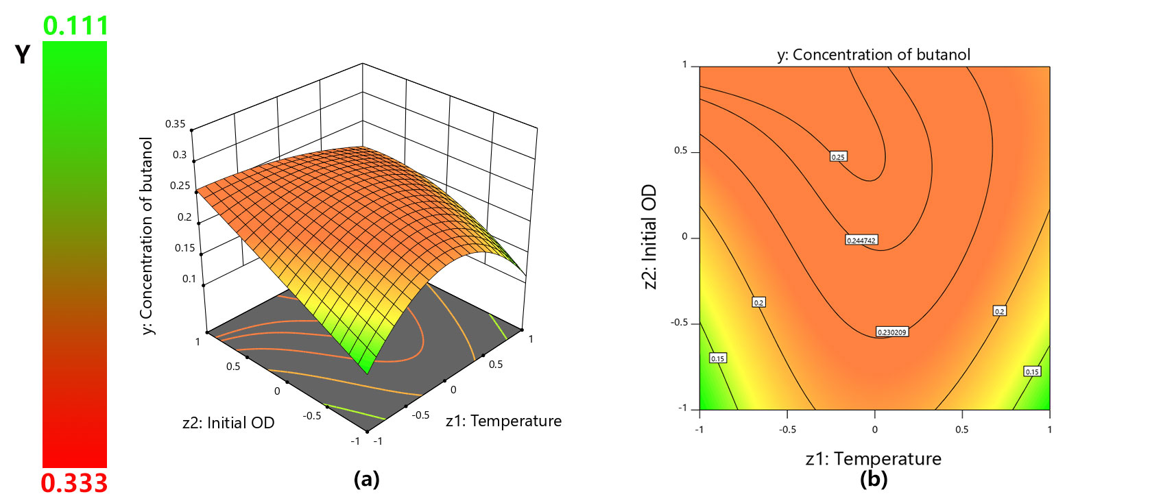
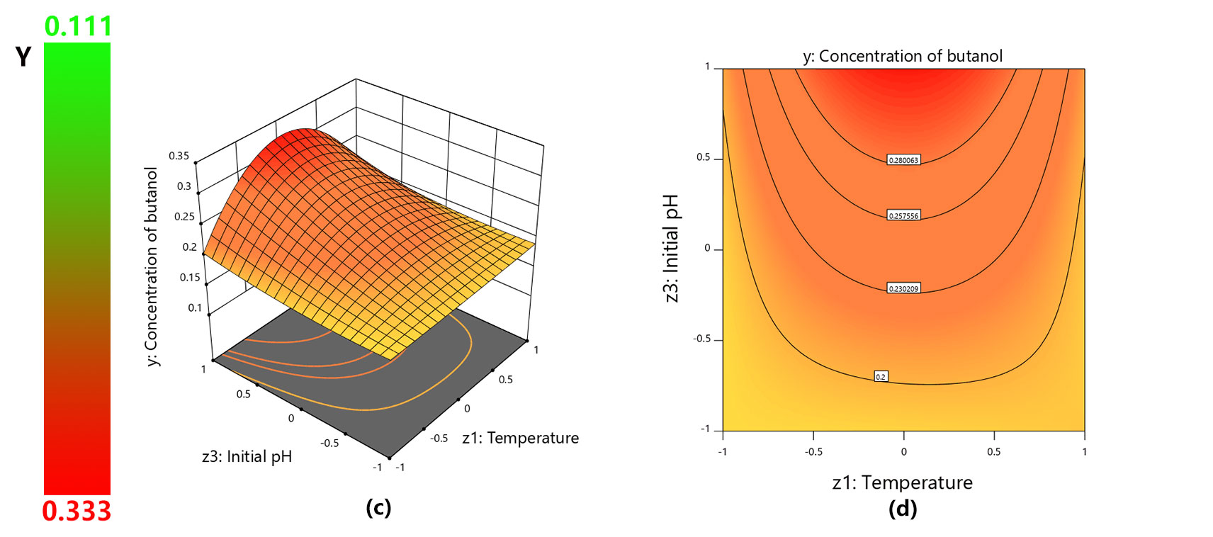
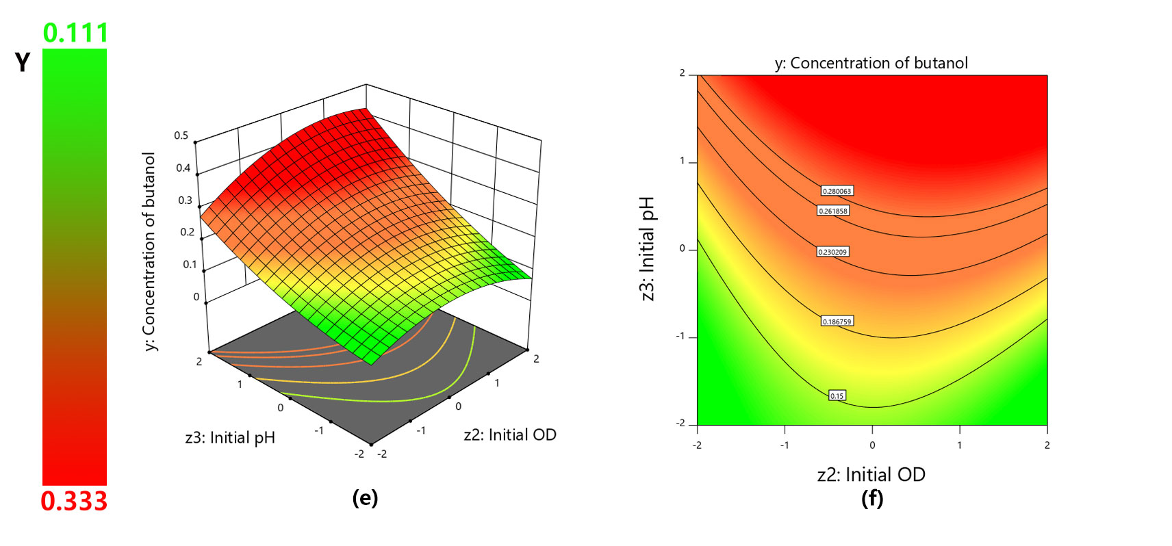Fig. 2 Response surface and contour plots for butanol production
2.4 Model verification

In order to verify the effectiveness of the optimization results, we conduct experiments again under the optimal conditions. We use Gompertz model to fit the experimental data. The verification results are shown in Fig. 3. Butanol reached a maximum of 0.406g/L after 26h, which was 52.35% higher than the butanol yield of control group. This shows that our model is effective in improving the butanol fermentation system.

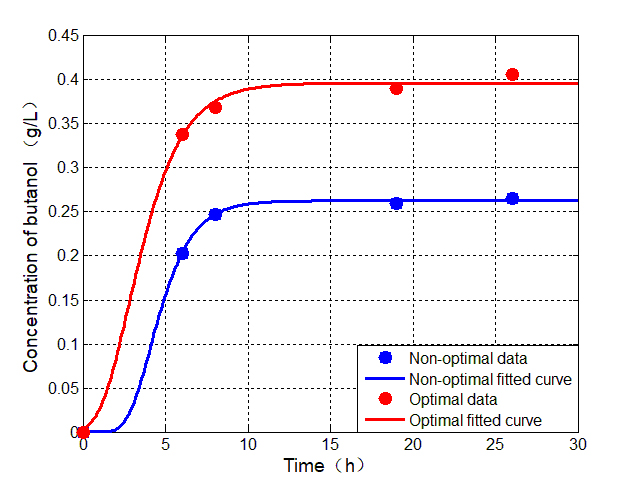Fig. 3 Comparison of butanol production between the optimal conditions and the non-optimal condictions. The non-optimal fermentation conditions are as follows: temperature is 37 ℃, initial OD is 11, initial pH is 7. The optimal fermentation conditions are as follows: temperature is 33.7 ℃, initial OD is 13, initial pH is 8.
3. Biochemical reaction model

We first consider each reaction as an independent system. We assume that the seven-step chain reaction in the fermentation process is consistent with the Michaelis-Menten equation. The basic model of biochemical reaction can be obtained according to the Michaelis-Menten equation and the law of conservation of mass [6]. The basic model was modified due to the competitive effects of different substrates on the same enzyme and the inhibition of the product. Using MATLAB 2014a to solve the above model, and the curve of the output of each product with time was obtained.
3.1 Basic theory

3.1.1 Michaelis-Menten equation

In biochemistry, the Michaelis-Menten equation is one of the most famous enzyme kinetic models. This model gives the relationship between the enzymatic reaction rate v and the substrate concentration [S] and enzyme concentration [E]. For the following enzymatic reactions:

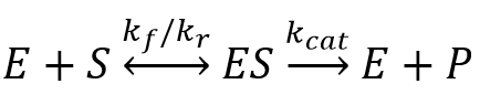Where，\({k_f}\)(forward rate)，\({k_r}\)(reverse rate)，\({k_{cat}}\)(catalytic rate) denote the rate constants; the double arrows between S(substrate) and ES(enzyme-substrate complex) represent the fact that enzyme-substrate binding is a reversible process, and the single forward arrow represents the formation of P (product).

When the enzyme concentration is much smaller than the substrate concentration, the product formation rate is:

\[\upsilon = \frac{{d[P]}}{{dt}} = \frac{{{k_{cat}} \cdot [S] \cdot [E]}}{{{k_m} + [S]}}\]

Where，[S] is the substrate concentration, [E] is the initial enzyme concentration, [P] is the product concentration.

3.1.2 Law of mass action

The law of mass action is: the rate of the elementary reaction is proportional to the power of the concentration of each reactant, where in the power exponent of each reactant concentration is the stoichiometry of the reactant in the reaction equation, and the proportional constant is called the chemical reaction constant. For the following biochemical reactions:

By the law of mass action:

\[\frac{{d[C]}}{{dt}} = - \frac{{d[A]}}{{dt}} = - \frac{{d[B]}}{{dt}} = J\]

\[J = k \cdot [A] \cdot [B]\]

Where，\(J\) is called flux of chemical reaction.
3.2 Basic model

At a constant concentration of enzyme, the Michaelis-Menten equation describes the relationship between reaction rate and substrate concentration. Therefore, The biochemical reaction from glucose to butanol shown in Fig. 4 can be described by equations (2)-(9).

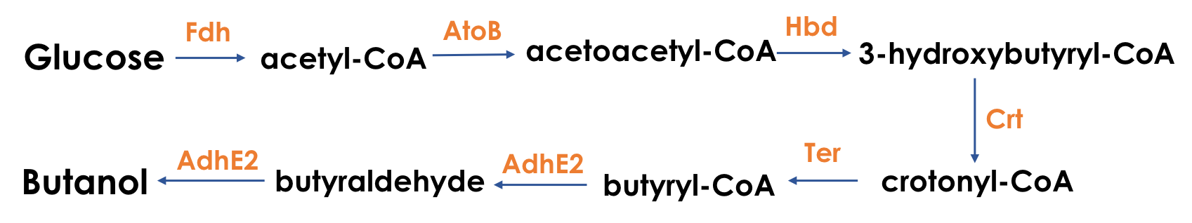Fig. 4 Biochemical pathway diagram of glucose to butanol

\[{v_{{x_1}}} = \frac{{d{x_1}}}{{dt}} = - \frac{{k_{cat}^{Fdh} \cdot {x_1} \cdot \left[ {Fdh} \right]}}{{k_m^{Fdh} + {x_1}}}\]

(2)

\[{v_{{x_2}}} = \frac{{d{x_2}}}{{dt}} = - {v_{{x_1}}} - \frac{{k_{cat}^{AtoB} \cdot {x_2} \cdot \left[ {AtoB} \right]}}{{k_m^{AtoB} + {x_2}}}\]

(3)

\[{v_{{x_3}}} = \frac{{d{x_3}}}{{dt}} = {v_{{x_2}}} - \frac{{k_{cat}^{Hbd} \cdot {x_3} \cdot \left[ {AtoB} \right]}}{{k_m^{AtoB} + {x_3}}}\]

(4)

\[{v_{{x_4}}} = \frac{{d{x_4}}}{{dt}} = {v_{{x_3}}} - \frac{{k_{cat}^{Crt} \cdot {x_4} \cdot \left[ {Crt} \right]}}{{k_m^{Crt} + {x_4}}}\]

(5)

\[{v_{{x_5}}} = \frac{{d{x_5}}}{{dt}} = {v_{{x_4}}} - \frac{{k_{cat}^{Ter} \cdot {x_5} \cdot \left[ {Crt} \right]}}{{k_m^{Ter} + {x_5}}}\]

(6)

\[{v_{{x_6}}} = \frac{{d{x_6}}}{{dt}} = {v_{{x_5}}} - \frac{{k_{cat1}^{AdhE2} \cdot {x_6} \cdot \left[ {AdhE2} \right]}}{{k_{m1}^{AdhE2} + {x_6}}}\]

(7)

\[{v_{{x_7}}} = \frac{{d{x_7}}}{{dt}} = {v_{{x_6}}} - \frac{{k_{cat2}^{AdhE2} \cdot {x_7} \cdot \left[ {AdhE2} \right]}}{{k_{m2}^{AdhE2} + {x_7}}}\]

(8)

\[{v_{{x_8}}} = \frac{{d{x_8}}}{{dt}} = \frac{{k_{cat2}^{AdhE2} \cdot {x_7} \cdot \left[ {AdhE2} \right]}}{{k_{m2}^{AdhE2} + {x_7}}}\]

(9)
3.3 Improved model

3.3.1 Competitive effects of two substrates on the same enzyme

Although we used the relationship between the Michaelis-Menten equation and the chain reaction to obtain the expression of butanol, the model only considered the case of single enzyme reaction. However, bifunctional acetaldehyde-CoA/alcohol dehydrogenase was used twice in the reaction, and different substrates competed for the enzyme. In this process, we assume that the substrate has no inhibition during the reaction.

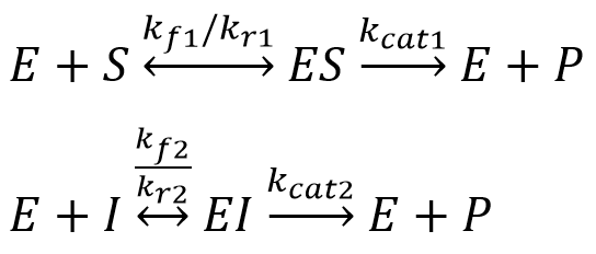As shown in the figure above, the two substrates combined to share the same enzyme can be approximated as a competitive inhibition kinetic equation:

\[\left[ {{E_f}} \right] = \left[ E \right] - \left[ {ES} \right] - \left[ {EI} \right]\]

(10)

\[{k_m} = \frac{{{k_r} + {k_{cat}}}}{{{k_f}}}\]

(11)

\[{k_1} \cdot \left[ {{E_f}} \right] \cdot \left[ S \right] = \left( {{k_r} + {k_{cat}}} \right) \cdot \left[ {ES} \right]\]

(12)

Equation (12) is based on the law of mass action, combined with equation (11), can obtain a model considering substrate competition:

\[{{\rm{v}}_{{x_6}}} = \frac{{d{x_6}}}{{dt}} = {v_{{x_5}}} - \frac{{k_{cat2}^{AdhE2} \cdot {x_6} \cdot \left[ {AdhE2} \right]}}{{k_{m1}^{AdhE2}\left( {1 + \frac{{{x_6}}}{{k_{m1}^{AdhE2}}}} \right) + {x_6}}}\]

(13)

\[{{\rm{v}}_{{x_7}}} = \frac{{d{x_7}}}{{dt}} = {v_{{x_6}}} - \frac{{k_{cat2}^{AdhE2} \cdot {x_7} \cdot \left[ {AdhE2} \right]}}{{k_{m2}^{AdhE2}\left( {1 + \frac{{{x_7}}}{{k_{m2}^{AdhE2}}}} \right) + {x_7}}}\]

(14)

3.3.2 Product inhibition

Because the product has an inhibitory effect on the reaction, the butanol concentration progress curve was fitted to equation (15).

\[v = \frac{{{k_{cat}} \cdot \left[ S \right] \cdot \left[ {\rm{E}} \right]}}{{{k_m} + \left[ S \right] \cdot \left( {{\rm{1 + }}\frac{P}{{{k_1}}}} \right)}}\]

\[{v_{{x_8}}} = \frac{{d{x_8}}}{{d{t_{}}}} = \frac{{k_{cat2}^{AdhE2} \cdot {x_7} \cdot \left[ {AdhE2} \right]}}{{k_{m2}^{AdhE2}\left( {1 + \frac{{{x_8}}}{{_{ki}AdhE2}}} \right) + {x_7}}}\]

(15)

where, P is the concentration of the reaction product and \(k_i^{AdhE2}\) is a product inhibition constant.

3.4 Model solving

We use MATLAB 2014a to solve the above system of ordinary differential equations. The following parameters were used:

Table 4 Parameters in chain reaction model of butanol production system

Parameter	Variable Name	Value	Reference
Michaelis Constant for Fdh	\[k_m^{Fdh}\]	0.0150mM	[7]
Catalysed rate of reaction for Fdh	\[k_{cat}^{Fdh}\]	3.3000s^(-1)	[7]
Michaelis Constant for AtoB	\[k_m^{AtoB}\]	0.4700 mM	[7]
Catalysed rate of reaction for AtoB	\[k_{cat}^{AtoB}\]	2.1000s^(-1)	[7]
Michaelis Constant for Hbd	\[k_m^{Hbd}\]	0.0187 mM	[8]
Catalysed rate of reaction for Hbd	\[k_{cat}^{Hbd}\]	35.1560s^(-1)	[8]
Michaelis Constant for Crt	\[k_m^{Crt}\]	0.1070 mM	[8]
Catalysed rate of reaction for Crt	\[k_{cat}^{Crt}\]	266.4300s^(-1)	[8]
Michaelis Constant for Ter	\[k_m^{Ter}\]	0.0027 mM	[7]
Catalysed rate of reaction for Ter	\[k_{cat}^{Ter}\]	91.0000s^(-1)	[7]
Michaelis Constant for AdhE2	\[k_{m1}^{AdhE2}\]	0.0230 mM	[7]
Catalysed rate of reaction for AdhE2	\[k_{cat1}^{AdhE2}\]	2.2000s^(-1)	[7]
Michaelis Constant for AdhE2	\[k_{m2}^{AdhE2}\]	0.4000 mM	[7]
Catalysed rate of reaction for AdhE2	\[k_{cat2}^{AdhE2}\]	2.9000s^(-1)	[7]
Inhibition constant for product	\[k_i^{AdhE2}\]	2.1 mM	[7]
Product concentration	\[{x_i}\]\[\left( {{\rm{i = }}1 \ldots 8} \right)\]	----

The results of the solution are shown in Fig. 5, where (a) is the curve of the concentration of each intermediate product, and (b) is the curve of the concentration of butanol.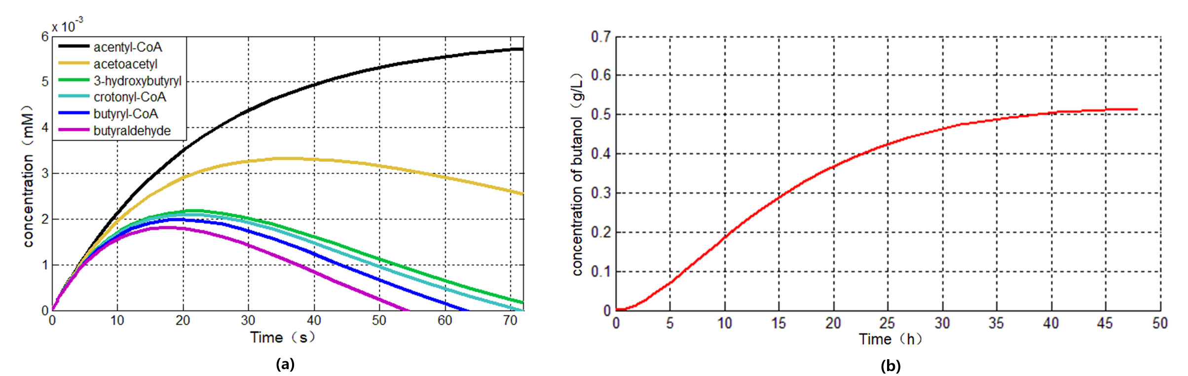

Fig. 5 (a) intermediate product curve(b)Butanol curve

As can be seen from Fig. 5(a), in the butanol fermentation reaction, the first step is the slowest, and the fifth, sixth, and seventh steps are faster, so the rate-limiting step of the reaction is the reaction of glucose to acetyl-CoA.

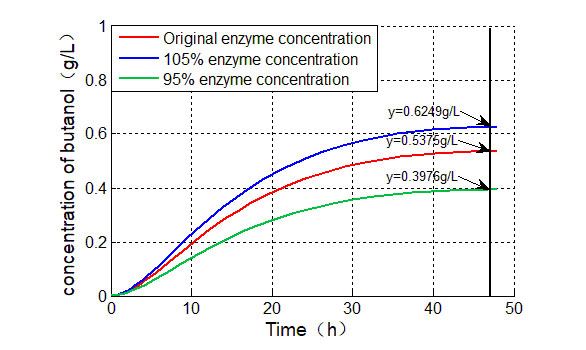Fig. 6 Butanol production at different enzyme Fdh concentrations

The simulated butanol change curve is shown in Fig. 5(b). We tried to increase the enzyme concentration of the reaction by 5% and reduce the enzyme concentration by 5%. The corresponding yield of butanol is shown in Fig. 6. When the enzyme concentration increased by 5%, the butanol production increased by 16.26%; when the enzyme concentration decreased by 5%, the butanol production decreased by 26.03%.

3.5 Sensitivity analysis

Finally, we performed a sensitivity analysis of the model parameters to determine the most appropriate parameters producing the best impact on butanol fermentation. Sensitivity analysis is performed by perturbing each parameter up and down by 5% and calculating the change in output relative to the parameter. The results of the sensitivity analysis are shown in the table below:

Table 5 Sensitivity analysis results when the parameters are perturbed up and down by 5%

Parameter	Variable Name	Butanol at 5% increase (g/L)	Butanol at 5% reduction (g/L)	Butanol production change ratio
Michaelis Constant for Fdh	\[k_m^{Fdh}\]	0.5483	0.4813	13.02%
Catalysed rate of reaction for Fdh	\[k_{cat}^{Fdh}\]	0.5144	0.5144	0
Michaelis Constant for AtoB	\[k_m^{AtoB}\]	0.5144	0.5144	0
Catalysed rate of reaction for AtoB	\[k_{cat}^{AtoB}\]	0.5144	0.5144	0
Michaelis Constant for Hbd	\[k_m^{Hbd}\]	0.5052	0.5238	3.62%
Catalysed rate of reaction for Hbd	\[k_{cat}^{Hbd}\]	0.5208	0.5076	2.57%
Michaelis Constant for Crt	\[k_m^{Crt}\]	0.5012	0.5282	5.25%
Catalysed rate of reaction for Crt	\[k_{cat}^{Crt}\]	0.5269	0.5011	5.02%
Michaelis Constant for Ter	\[k_m^{Ter}\]	0.4869	0.545	-11.29%
Catalysed rate of reaction for Ter	\[k_{cat}^{Ter}\]	0.5378	0.4908	9.14%
Michaelis Constant for AdhE2	\[k_{m1}^{AdhE2}\]	0.5103	0.5186	-1.61%
Catalysed rate of reaction for AdhE2	\[k_{cat1}^{AdhE2}\]	0.517	0.5116	1.05%
Michaelis Constant for AdhE2	\[k_{m2}^{AdhE2}\]	0.5144	0.5144	0
Catalysed rate of reaction for AdhE2	\[k_{cat2}^{AdhE2}\]	0.5144	0.5144	0
Inhibition constant for product	\[k_i^{AdhE2}\]	0.5168	0.5118	0.97%

From the sensitivity analysis, it can be seen that the Michaelis constant \(k_m^{Fdh}\) of the rate-limiting reaction is the most sensitive parameter. By changing the initial pH and temperature to the optimal value of the parameter \(k_m^{Fdh}\), the yield of butanol in the system can be effectively increased.

4. References

[1]Yachun S. Optimization of butanol fermentation and kinetic analysis by Clostridium BeijerinckII F-6[D]. Harbin :Harbin Institute of Technology,2017:23-39.

[2]Shukor H, Al-Shorgani NKN, Abdeshahian P, Hamid AA, Anuar N, Rahman NA & Kalil MS. 2014. Production of butanol by Clostridium saccharoperbutylacetonicum N1-4 from palm kernel cake in Acetone-Butanol-Ethanol fermentation using an empirical model[J]. Bioresource Technology, 170:565-573.

[3]Ming G, Bin F & Yu G. SHIYAN SHEJI YU RUANJIAN YINGYONG[M]. Beijing: Chemical Industry Press, 2017.

[4]Wang Z, Cao G, Jiang C, Song J & Zheng J. 2013. Butanol production from wheat straw by combining crude enzymatic hydrolysis and anaerobic fermentation using Clostridium Acetobutylicum ATCC824[J]. Energy & Fuels, 27:5900-5906.

[5]Wang Y & Blaschek HP. 2011. Optimization of butanol production from tropical maize stalk juice by fermentation with Clostridium Beijerinckii NCIMB 8052[J]. Bioresource Technology, 102:9985-9990.

[6]Hao G & Hong Q. SHUXUE DONGLIXUE MOXING[M]. Beijing: Peking University Press, 2017.

[7]BRENDA[DB/OL]. http://www.brenda-enzymes.org/index.php,2018.9.15.

[8]Davis MA. Exploring in vivo biochemistry with C4 fuel and commodity chemical pathways[D]. Berkeley: University of California, Berkeley, 2015:23.

Team:UESTC-China/Model butanol

1. Introduction

2. Optimization of butanol fermentation process

3. Biochemical reaction model

4. References