Team:UNSW Australia/Model/EKD

Enzyme Kinetics and Diffusion
Why Make a Mathematical Model?
Previous experiments involving enzyme scaffolding have shown various yields, ranging from fractional improvement to 77-fold increases in product titre 2,7. The exact improvements on reaction efficiency made via scaffolding enzymes vary across experiments. Notably, different scaffolds, enzymes, and substrates may result in significantly different yields 2. We are employing the enzymes used in Indole Acetic Acid synthesis in our system, utilizing their kinetic parameters to dictate the model. Additionally we model the taxol synthesis pathway as it is a potential commercial application of our scaffold. We consider the diffusion of the intermediary substrate when the enzymes are placed various distances apart. We believe the model was able to assist in our understanding of how scaffolding enzymes can alter reaction efficiency.
Aim of Modeling
We aimed to model the effect of distance between enzymes on reaction efficiency, hypothesizing that co-localising enzymes would increase reaction efficiency by decreasing intermediary loss to diffusion. Under this model, we assumed that intermediary loss to diffusion is significant enough to limit rates of product formation. We further aimed to incorporate the specific kinetics of enzymes in our system, and create an adaptable model that could generate data for other enzyme reaction pathways.
Boundary Conditions
To define the scope of the model, some initial boundary conditions were required. The boundary conditions are as follows, with justification following:
- The first enzyme produces the second substrate at a constant rate.
- The enzymes are some distance 0 < R < ∞ apart (they are not touching, nor are they infinitely far apart).
- The rate of production of the final product is dependent on the concentration of the second substrate that diffuses to enzyme B.
- The enzymes are not points, but rather small spheres given the size of the enzymes relative to the distance between them.
- The reactant can escape to infinity.
Condition (1) creates a linear diffusion gradient for the second substrate’s diffusion to enzyme B. This follows Fick’s Law of diffusion 4. In order to meet this condition the concentration of the first substrate must be held constant. Since the first substrate is being consumed by enzyme A, it must be kept in flow to the system.
Condition (2) describes the physical nature of the system; the enzymes attached to prefoldin are a finite distance apart.
For Condition (3), the second enzyme functions as a sink, removing S2 particles from the system and creating the final product IAA. Similarly the rate of reaction for enzyme B is dependent on the concentration of substrate 2 present; as with any enzyme reaction, thus it is a first order sink 6.
Condition (4) is important to define the diffusion gradient and was verified by the molecular dynamics simulations.
The final condition determines how the model treats the concentration of substrate at very large distances from the source enzyme. Allowing the substrate to escape to infinity implies the concentration tends to zero as distance tends to infinity. This avoids the complexities of determining how long it might take for the reaction to complete by considering the probability of the prefoldin-enzyme complex and escaped substrate colliding due to random walk 3.
Enzyme Kinetics
The IAA reaction is a 2-step sequential reaction:
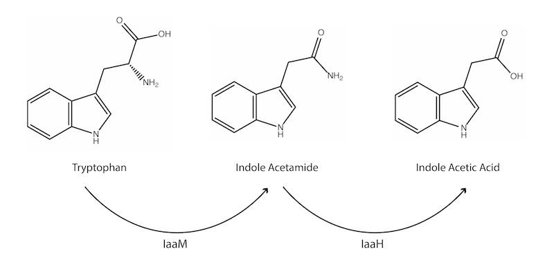
Figure 1: The enzymatic patway for the production of IAA.
Each enzyme interacts with a single substrate to produce a single product, and each enzyme has its own set of kinetic parameters. We employed the indole acetic acid pathway as a model enzyme reaction, as the enzymes are readily available with well-defined kinetic parameters.
The Michaelis-Menten (MM) equation (equation 1) describes the kinetics of an enzyme-substrate interaction under a given set of environmental conditions. MM kinetics were used to describe the effective rates of product formation and consumption at each enzyme in the sequential reaction.
The Km or Michaelis constant is an affinity constant for the particular enzyme-substrate interaction, whilst the Vmax is the maximum speed of the enzyme when substrate concentration is saturated. The equation is pseudo first order in this sense, as substrate concentration is high, enzyme speed (V) approaches Vmax, but whilst it is low, the MM equation holds true.
To simplify the model, we assume that the first substrate (tryptophan) is maintained in the system at a constant, saturating concentration, thus the first enzyme produces the second substrate (IAM) at a constant rate. This leads to a simple, linear diffusion of IAM from enzyme A. Thus, the production rate at enzyme A of substrate 2 is simply the Vmax of enzyme A (equation 2).
During consultations with industry about our model, the idea of keeping the first substrate in constant supply to the system arose. Dr Warren King suggested that it would be preferable in a commercial setting, as continuous systems generally make more efficient use of resources. Dr King also confirmed it would simplify the remainder of our analysis in developing the model.
Fick’s law is used to describe the diffusion of IAM from enzyme A into the system in two dimensions (equation 3).
Where J is the diffusion flux in amount per unit area per unit time, D is the diffusivity in area per unit time, and ϕ denotes the concentration in amount per unit volume. The driving force of diffusion using Fick’s law is a concentration gradient. The concentration gradient in this model is determined by the difference in production and consumption of substrate 2 between the first and second enzyme. Thus the rate of substrate consumption at the second enzyme will determine the diffusive flux toward second enzyme.
We define the second enzyme in the system as the sink for diffusion, with consumption rate a 1st order reaction defined by the Michaelis-Menten equation. At the edge of the second enzyme (represented by E4 on the diagram), the consuming boundary condition is defined by equation 3.
Vmax and Km are now specific to the second enzyme; indole acetamide hydrolase. As the substrate needs to diffuse from enzyme A, the concentration of substrate reaching enzyme B is expected to be low, therefore the reaction rate at the second enzyme is dependent on the amount of substrate reaching enzyme B through diffusion. Thus the 1st order form of the Michaelis-Menten equation applies.
Our System
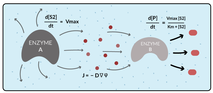
Figure 2: Diffusion of substrate from Enzyme A to Enzyme B.
Assumptions of This Model
At each enzyme, employing the Michaelis-Menten equation assumes the law of mass action, meaning all substrate that reaches the boundary at each enzyme is completely converted to product 5. In reality, product levels are expected to be slightly lower than predicted due to imperfect substrate-enzyme interactions.
Employing Fick’s law of diffusion assumes that a concentration gradient is the only force driving substrate motion in the system. In reality, charge interactions may create a substrate channelling effect, or substrate-enzyme repulsion, leading to increased or decreased true product yields when compared to the predicted data 8. Fick’s law also does not account for the shape of each molecule, and how angular momentum of each of the substrate may affect motion of the substrate between enzymes 9.
The distance between enzymes is assumed to be relatively constant as the reaction takes place. In reality, the enzymes may be moving rapidly and non-constantly, creating variation in the amount of product produced over a given time 9. By employing a constant distance model we are effectively taking an average of the distance between enzymes.
Simplifying the geometry to 2 dimensions, and a half sphere further assumes that diffusion would not be biased in any directional plane in the real system. This assumes an equal and opposite flux in the plane perpendicular to the plane of distance between enzymes.
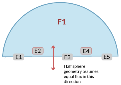
Figure 3: Geometry of the model developed in MATLAB looking at diffusion.
Approximating the enzymes as spheres is the last assumption employed to simplify the system, the enzymes are approximated as spheres as opposed to points due to the size of the enzymes relative to the distance between them (either reference MD or reference trigonometric analysis). Additionally, the exact position of the active site of the enzyme is not considered in this case. This may have an effect on the accuracy of the model in cases where the active site of the enzyme is pointed away from the next enzyme in the reaction pathway 2. A more realistic model would involve assigning the site of reaction (production or consumption) to be a point on each of the half-spheres. The point could then move over the surface of the half sphere, mimicking the changing orientation of the active site in a real enzyme reaction. This was not possible due to an inability to assign point-node boundary conditions on element meshes in MATLAB, however other more specialised software for solving finite element problems may be available to solve this problem.
Analysis and Results
The concentration of substrate reaching the sink over a 0.2 second time-frame was measured at multiple distances. The largest distance between enzymes was 1500 angstroms, with the smallest distance measured being 50 angstroms. The distance between enzymes was reduced by 50-angstrom increments to measure the effect of distance on final product yield. The model predicts a 5-fold improvement in IAA production when the enzymes are clustered together using prefoldin, compared to when they are free in solution (Figure 4).
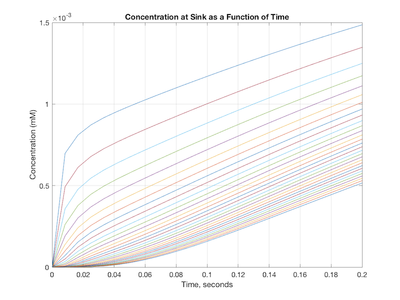
Figure 4: From left to right, each graph represents a smaller distance between the two enzymes. The uppermost graph presents the concentration-time curve when the enzymes are separated by a distance of 50 angstroms, with the lowermost graph displaying the concentration-time curve for a distance of 1500 angstroms.
The graphs show a faster achievement of steady-state IAA production when the two enzymes are clustered together, and higher overall concentration of the second substrate at enzyme B.
By integrating under each curve, we calculated the amount of product formed at each distance over the same time period (Figure 5). As stated above, this calculation assumed perfect substrate to product conversion.
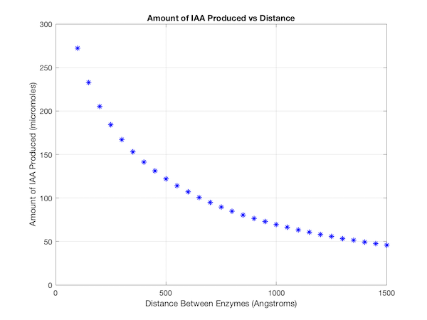
Figure 5: Each point represents the amount of IAA produced in micromoles when the enzymes are separated by a certain distance in angstroms.
We were less concerned with the exact values of product generated by the model, and more with the relationship between distance and amount of product formed. From this result the relationship between distance and product formation was made clear; product formation increases non-linearly as the separation between enzymes is reduced.
Taxol Synthesis
We met with Prof. Groundwater to discuss the potential of commercialising our scaffold who suggested that we look into the side-chain synthesis of Taxol as a potential application. We employed the kinetic parameters for the taxol enzymes in our mathematical model to control the rate of production and consumption of substrate at each enzyme. We found that clustering the enzymes on prefoldin resulted in an approximate 6-fold increase in taxol side-chain production (Figure 6).
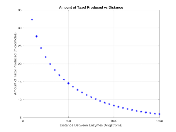
Figure 6: Each point represents the amount of Taxol produced in micromoles when the enzymes are separated by a certain distance in angstroms.
MATLAB
The MATLAB PDE toolbox was used to solve the system. The overall workflow involves generating a geometry of the model, creating a mesh, and solving the equations at relevant nodes in the mesh. For example, at the nodes surrounding the first enzyme, the flux value, J, is set to be the rate of production of the first enzyme based on Michaelis-Menten Kinetics. Whilst at the second enzyme, the flux value is set to be the rate of consumption of the second enzyme based on Michaelis-Menten Kinetics. The files for generating the geometry and solving the system are available here, with a MatlabREADME.txt file supplied to describe how the model can be manipulated. An example mesh for the two enzymes is shown (Figure 7).

Figure 7: A solved mesh of our geometry. The half circle on the left represents the source, while the half circle on the right represents the sink. The tetrahedral elements that form the mesh make up the nodes; each side of the tetrahedral elements joins at a node. The values of x and y correspond to the units used to build the geometry of the system. In this case, the enzymes are set 2 units from the center at x values of -2 and 2, whilst the radius of the half sphere is set to 4 units. The z value corresponds to the concentration of substrate, creating the 3D image.
From this mesh, the concentration of substrate at various nodes can be extracted. This allows for the generation of graphs of concentration versus time, and concentration versus distance, amongst others. Thus we employed the finite element method to solve our system, utilising MATLAB to numerically solve the system.
Reflections
Overall, the model served to effectively support our initial hypothesis that reduced distance between enzymes would increase product yield. We believe the boundary conditions and assumptions do not limit the possibility of validating the model against experimental data. However, we did not reach the stage in building our prefoldin scaffold where such validation was possible. Thus the model served mainly to verify our design process, and could not be modified based on experimental results. Furthermore we believe there is better-suited software specialised for designing molecular meshes and solving numerical problems, such as the FeNics toolkit. Ultimately we would like to expand the model to account for varied enzyme stoichiometry in the geometry of the model. Currently stoichiometry can be included by changing the rate of production or consumption at the sink or source. For example if one wanted to include a second consuming enzyme, it could be implemented by doubling the rate of consumption at a single sink, however this is an approximate method. Additionally in future we would like to incorporate the effects of electrostatic interactions that can occur between enzymes and substrates. Such interactions can create 'channeling' effect and have been postulated as the cause of some of the extremely large improvements in yield recovered from enzyme scaffolding systems 2. Due to inexperience in computational mathematics, we were not able to incorporate some of these more complex features in our model.
References
- Busse, C., Kache, A., and Wagner, S. Boundary Conditions: What They Are, How To Explore Them, Why We Need Them, and When To Consider Them. Organisational Research Methods. 20 574-609 (2017).
- Castellana M. et al. Enzyme clustering accelerates processing of intermediates through metabolic channeling. Nat Biotechnol. 32 1011-1018 (2015).
- Gaudillière, A. Collision probability for random trajectories in two dimensions. Stochastic Processes and their Applications. 119 775-810 (2008).
- Janavicius A.J., and Poskus A. Nonlinear Diffusion Equation with Diffusion Coefficient Directly Proportional to Concentration of Impurities. Acta Physica Polonica. 107 519-524 (2004).
- Murray, J.D. Mathematical Biology: I. An Introduction Springer. 3 (2002).
- Uddin N. Enzyme Concentration, Substrate Concentration and Temperature based Formulas for obtaining intermediate values of the rate of enzymatic reaction using Lagrangian polynomial. International Journal of Basic and Applied Sciences. 1 299-302 (2012).
- Whitaker, W.R and Dueber, J.E. Metabolic pathway flux enhancement by synthetic protein scaffolding. Methods Enzymol. 497 447-468 (2011).
- Eun, C., Kekenes-Huskey, P., Metzger, V., and McCammon, J. A model study of sequential enzyme reactions and electrostatic channeling. J Chem Phys. 140 (2014).
- Rice, S.A. Comprehensive Chemical Kinetics. Diffusion-Limited Reactions Elsevier, Amsterdam 25 39-45 (1985).