
Team:Stockholm/Model


Model
Modeling was an integral part of our project, leading to some of our most important achievements:
- Accurately predicting the behavior of our laccase in the lab using Quantum Mechanical calculations and Molecular Dynamic simulations
- Creating a new model to accurately calculate the rate of the reaction (kcat) for several substrates and mutants of a wider range of monooxidases
- Writing a handbook in molecular modeling for iGEM projects
- Using the created model of the enzyme to understand, learn and create a mutant laccase, as well as explain its behavior
Introduction
Our project heavily relies on modeling for both analysis, and as the basis for the development of a mutant enzyme with antibiotic degrading properties. The utilization of molecular models to understand miniscule events that together build the whole degradation reaction is crucial for this kind of rational enzyme development. Our aim with the use of modeling can be broken down into two parts:
- To use modeling to predict and analyze molecular behavior with sophisticated molecular modeling techniques.
- To show how modeling can be used to predict and analyze molecular behavior with sophisticated molecular modeling techniques and spread this within the iGEM competition.
To achieve the first goal - developing an enzyme for degrading a set of antibiotics in wastewater - we have used rational enzyme design. To do this, we employed three molecular modeling methods
- QM (Quantum Mechanics) for reaction characterization
- QM/MM (Quantum Mechanics/Molecular Mechanics) for analysis of substrate/enzyme association
- and MD (Molecular Dynamics) for structural analysis.
The more you understand about your system chemically, the easier you can solve your problem.
As for the second goal, we created a Handbook in Molecular Modeling. We have made the whole handbook available on our wiki as our contribution to the iGEM community, and hope that it will be used by future teams. If you are using the handbook, please cite it on your model page.
Background
The basis for our modeling was molecular modeling, which is based on a combination of different mathematical models, involving both physical chemistry and QM.
Quantum Mechanics
QM is a very accurate representation of the miniscule events that make up the universe. The equations that we used are different versions of the Schrödinger equation.
$$ i\frac{\hbar}{2\pi}\frac{d\Psi}{dt} = H\Psi \mathrm{, where} \left | \Psi \right |^2 = \varrho \mathrm{,\ and\ } $$ $$ \varrho\ \mathrm{is\ the\ probability\ density, i.e.} \int \int \int \left | \Psi \right |^2 =P_V $$where P is the probability of finding the particle within the volume defined by the integration volume V. The interesting quantity here is H, the Hamiltonian, which is an energy matrix (a matrix for which the states of a system comprise the eigenvectors and the energies of each are the corresponding eigenvalues). In mathematical terms, this is:
$$ H\Psi = E\Psi $$Determining the Hamiltonian is thus crucial for determining important factors about the system. For electronic systems, the Hamiltonian can be expanded in five terms: nuclear-nuclear repulsion, nuclear kinetic energy (approximated to be zero under the Born-Oppenheimer approximation) nuclear-electron attraction, kinetic energy and electron-electron repulsion:
$$ H = E_{n-n}+E_{n-e}+E_{e-KE}+E_{e-e} $$When you have a Hamiltonian as a function of the spatial coordinates from which we can determine its eigenvectors, we can identify the eigenvectors with the spin orbitals of the system. However, upon constructing the Hamiltonian, we encounter a problem. The last term of this equation, the electron-electron repulsion, is inherently dependant on the eigenvectors of the very Hamiltonian we are trying to determine. Therefore, we have to employ numerical methods to estimate this factor. Throughout the modeling, we have used a DFT level of theory. This means that we call the electron repulsion term a functional of the electron density ($E_{e-e}(\varrho)$), and iterate until we get a self-consistent field.
Thermodynamics
Thermodynamics heavily influenced us in coming up with how the system behaves. Thermodynamics has to be used to make sense of the energies and the system that are created. The basic equation for the qualitative evaluation of the system is the equation for the Gibbs free energy:
$$ \Delta G = \Delta H - T \Delta S, \mathrm{where\ T\ is\ constant} $$ $$ \delta G = \delta H - T\delta S - \delta TS, \mathrm{where\ T\ is\ variable} $$While we can calculate the chemical energy in a system very accurately using QM, our system is not perfect and does not only exist in the state that we calculated for. In truth, the system can occupy a number of states (W). However, the occupancy of each state varies according to a Boltzmann distribution ($e^{-\frac{E}{RT}}$) across all states with different energies E. This phenomenon is called entropy and is defined as:
$$\Delta S = k_B ln\textrm{W}$$This was a leading thought throughout our modeling - how can we describe the system’s behavior not only in one conformation but in all conformations?
Reaction Kinetics and Electron Transfer
We knew very early on that the reaction we considered was an electron transfer (ET), which is governed by the Marcus equation for ET:
$$ k_{ET(A > B)} = k*\left | V_{AB} \right |^2e^{\frac{(\Delta G-\lambda)^2}{4\lambda k_BT}} $$This governs how fast the electron transfer occurs, and depends on three factors:
- $\Delta G$, which is the energy difference between the initial and final states of the transfer.
- $\lambda$, the reorganizational energy during transfer.
- $V_{AB}$, the electronic matrix coupling element, or the geometric overlap between the donor and acceptor orbitals (how close they are in space). This factor is highly distance-dependent, which can be used to improve the model as seen in the methods and results page.
Molecular Mechanics
QM is the deepest level of theory as mentioned, that can only use for very small systems. These small systems can be of any type and any complexity in the electronic configuration (for example if we introduce ions or heavy atoms). In biological systems (proteins, DNA) however, we do not have such complexity. Rather, we handle very similar bonds (peptide chains) with similar properties. Also, since most of the time no bonds are formed or broken, we can assume a spring-like behavior of each bond. Accounting for charges and Van der Waals radii, we can create a fully classical simplified model of very large systems.
$$ V_{\mathrm{AMBER}} = \sum_{i}^{n_{\mathrm{bonds}}}b_i(r_i-r_{i,eq})^2+\sum_i^{n_{\mathrm{angles}}}a_i(\theta_i - \theta_{i,eq})^2 $$ $$+\sum_i^{n_{\mathrm{dihedral}}}\sum_n^{n_{\mathrm{i},\mathrm{max}}}(\frac{V_{i,n}}{2})[1+\mathrm{cos}(n_i-\gamma_{i,n})] $$ $$+\sum_{i < j}^{n_{\mathrm{atoms}}}(\frac{A_{ij}}{r_{ij}^{12}}-\frac{B_{ij}}{r_{ij}^6})+\sum_{i < j}^{n_{\mathrm{atoms}}}\frac{q_iq_j}{4\pi\epsilon_0r_{ij}} $$The equation above describes the classical Hamiltonian, or the energy of the system according to the Amber force field. Calculating the energy gradient (forces) shows in what direction the system will evolve over time. Because every bond is different, the parameters (bi, ai, Aij and so on) are determined experimentally or using a more complex level of theory. Since they are only accurate for very specific systems under non-extreme conditions, we cannot use them in extreme conditions. Because of this, parameters already exist for amino acids that do not interact strongly with other residues. This kind of model can be used to simulate a large-scale system over time, for example, protein folding, DNA annealing/melting, or substrate/binding pocket dynamics.
Methods
While there is a lot of code involved, we have chosen to describe what we did in this section, rather than exactly which commands we used or the detailed theory behind everything. For this, please read the corresponding sections in the handbook provided. For all calculations, the supercomputer Kebnekaise at HPC2N, Umeå University in Sweden was used.
For our model to be successful, we needed to understand how our system behaves, functions, interacts with its environment and, perhaps most importantly, how we can alter the system to improve a set purpose.
Our project revolves around a laccase from Trametes versicolor, which we want to use to inactivate sulfamethoxazole (SMX). However, this laccase is not suitable for wastewater treatment due to its low efficiency at the moment. This enzyme has been shown to require from several hours to days for a significant degradation of SMX. We wanted to improve this degradation rate using rational enzyme design. In order to do that, we needed to understand how the system works and what our system (i.e. the laccase) does when we introduce the substrate or mutations. In this way, we integrated our model with the wet lab work in both the developmental (mutating the enzyme) and analytical aspects (deciding which tests to perform). Afterwards, we can assess the accuracy of the model to further understand the system.
In short, our modeling can be broken down into two sections:
- Understanding the system
- The reaction
- The Dynamic Properties
- Optimizing the reaction
Understanding the system
The dynamic properties
Our enzyme of choice, the laccase, has some very interesting properties. As Jones and Solomon (year) stated: “It is fascinating to consider that while laccases and other MCOs [multicopper oxidases] have nearly identical Cu active sites they exhibit substantial diversity in substrate interactions and catalytic rates.” This, along with the other above mentioned clues, led us to believe that the enzyme could be developed to degrade our specific antibiotic (SMX). First of all, we needed to figure out what led to this behavior.
Firstly, we aligned the PDB structure of our protein of interest (1GYC) with a similar one (1KYA) that had an affinity for a compound very similar to ours - namely xylidine. The similarity is in the aminophenyl group, which seems to fit in the binding pocket (even though experimental data showed higher affinity to more heavily phenylated compounds, such as lignin). This is shown in Figure 1.
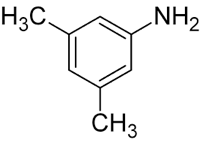
Figure 1. SMX (left) and Xylidine (right). The similarity can be seen in the leftmost group on SMX.
We could thus place the SMX in a similar position in the active site using Avogadro, a molecule viewing and structural editing program. To figure out the dynamics of the protein with SMX bound, we first needed to find the parameters to the Amber force field to a couple of unusual groups. This was done using the quantum mechanical software called Gaussian, and dividing the four different copper geometries into different sections and finding the parameters separately using B3LYP 6-31G(d’,p’) level of theory (see the handbook for commands used). Performing optimization (for equilibrium parameters) followed by a frequency calculation finds all the necessary parameters. For frequency calculations, the force constants were extracted using the mcpb.py routine.
The PDB-files were then renumbered in terms of residues according to the separations during parametrization. The regions used for this can be seen in Figure 2.
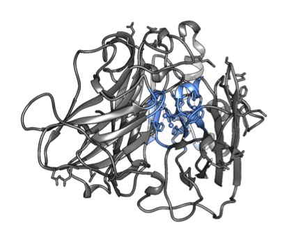
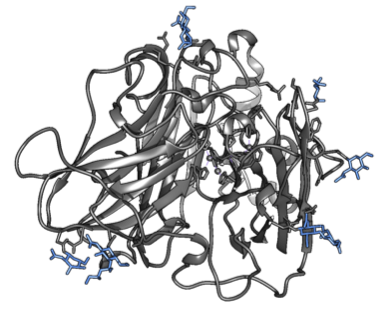
Figure 2. The copper-histidine complexes within the enzyme (left) and the glycosylations on the surface (right). The groups are highlighted in blue.
By positioning SMX in a couple of starting positions and constructing separate parameters for possible $\pi$-stacking (non-bonded), we could run a molecular dynamics simulation to figure out how the dynamic system would look. Keep in mind that the spontaneity of a process is dependent on both the bonded energy and the entropy of the system. The system equilibrated and converged nicely into folded structures not far off from the original crystal structure (1GYC), as you can see in Figure 3.
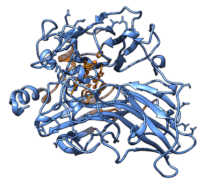
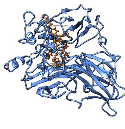
Figure 3. Snapshots of the molecular dynamics simulations over approximately 0.3 ns for the system without SMX (left) and with SMX (right). The commands for these calculations can be seen in appendix 1, and the additional parameters used can be seen in appendix 2. The added orange residue on the right is SMX, which it says in a very small font.
From the MD simulations SMX has too small inertia to stabilize the highly fluctuating phenylalanine residues at positions 162, 332 and 337 (see Video 1 further down the page). A hydrogen bond between the aspartic acid residue at position 206 and SMX seems to be possible with smaller distances, but when some of the distances are as high as 15Å, it is highly unlikely that it is formed under these conditions. We can see from the vivid translatory motion of the phenylalanine residues that the entropy for the enzyme is significantly lower for the bound system than for the unbound state. Now, having understood the association qualitatively, we need to put it into quantitative measures. To do this, we need to consider the first step of the reaction, that will be referred to as association:
$$ \mathrm{SMX} + \mathrm{Laccase} \rightleftharpoons \mathrm{SMX-Laccase} $$The equilibrium constant, $K_D$, determines the ratio of the product to the product of the reactants:
$$ K_D = \frac{[\mathrm{SMX-Laccase}]}{[\mathrm{Laccase}]*[\mathrm{SMX}]} $$which is also, according to the Nernst equation:
$$ \Delta_r G^o = -RTln(K_D) \iff K_D = E^{-\frac{\Delta_rG^o}{RT}}\mathrm{, where } $$ $$ \Delta_r G^o = \Delta_r G^o_{\mathrm{SMX-Laccase}} - \Delta G^o_{\mathrm{SMX}} - \Delta_r G^o_{\mathrm{Laccase}} $$We can thus, by calculating the individual values of $\Delta G^o$ calculate the $ \Delta_r G^o$ and arrive at a value for $K_D$. To do that, we need to be able to account for the difference in ΔG upon association. This difference would be due to the interactions that cause the substrate to associate with the binding pocket. Without an empirical hydrogen bonding database or other classical, cost-effective approaches, we cannot accurately estimate the strength and nature of these interactions, especially when the substrate is interacting loosely with the copper clusters. In this case, we chose to use QM/MM, and treat the active site along with the substrate quantum mechanically. The rest of the huge system can be somewhat accurately modeled using classical methods since we do not expect a big difference in the MM-regions. The results from the QM/MM calculations can be seen below. The Amber-Gaussian interface was used, which is outlined in the handbook.
Table 1. $\Delta G$ values calculated as the total energy of three separate systems, as described in the table. Also, the total $\Delta_r G$ calculated as $\Delta G^o_{SMX-Laccase} - \Delta G^o_{SMX} - \Delta G_{Laccase}$ is shown below.
| System | $\Delta G^o$ (a.u.) | $\Delta G^o$ (J) | Level of theory |
|---|---|---|---|
| SMX bound to Laccase, solvated | -13367.466 | -5.8280e-14 | 6-31G PBE0 |
| SMX, solvated | -1200.058 | -5.23203e-15 | 6-31G B3LYP |
| Free laccase, solvated | -12162.2314 | -5.3025e-14 | 6-31G B3LYP |
Meaning that the $\Delta_r G^o $ of the reaction is $\Delta_r G^o = -2.2975131*10-17 J$ per single reaction. Exchanging $R$ for Boltzmann's constant ($k_B$) gives the equation: $$ K_D=e^{-\frac{rGo}{k_{B}T}} =e^{5584.163626} $$
... which is a very large number, that is completely unreasonable. What is noticeable, however, is that a slight change in any of the energy values contributes to a huge difference in the $\Delta_rG^o$, since the difference is down to a number of decimals small, as the total energies of the full systems are much less. The percentual accuracy has to, therefore, be tremendously high for these calculations to work. Due to time constraints, we could not get a better value, however, for future experiments looking at a smaller system (now the systems were solvated with explicit water molecules) by the use of QM/MM-PBSA, to get smaller fluctuations in the total energy, and thus get more reliable values.
With better values, we could have determined a $K_M$ value for the conformations applied in the mutated laccase. We also got a good perception of which binding modes are more effective versus less effective. To connect this to a $K_M$ value that could be measured using Michaelis-Menten kinetics, however, we needed to consider that the definition of $K_M$ differed somewhat from the definition of $K_D$:
$$ K_D = \frac{k_{\mathrm{association}}}{k_{\mathrm{dissociation}}} \mathrm{, while\ } K_M = \frac{k_{\mathrm{dissociation}}}{k_{\mathrm{association}}+k_{\mathrm{cat}}}$$$k_{\mathrm{association}}$ and $k_{\mathrm{dissociation}}$ are the rate constants for the associative reaction when SMX binds to the binding pocket of the laccase, upon which the reaction happens. For us to be able to infer a $K_M$ value from the $\Delta G$ without having to calculate the individual rate constants $k_{\mathrm{association}} \gg k_{\mathrm{dissociation}}$. In an MD simulation, this could be gauged by looking at the steric clashes and hindrances association of a substrate has and whether that activation energy association is much lower than the activation energy for the reaction. Then, the following approximation would be valid:
$$ K_D \approx \frac{1}{K_M} \approx e^{-\frac{\Delta G}{RT}} \iff K_M \approx e^{-\frac{\Delta G}{RT}}$$In other pages on the wiki, this is referred to as the $\frac{K_D}{K_M}$-approximation, and we have to show that it is valid later to use it. In short, we now understood how the substrate binds into the binding pocket.
1.2 The Reaction
However, the question remained on how the reaction takes place and how SMX reacts with the enzyme. Another key question was which of the many binding modes we saw earlier were productive binding modes. Thankfully, previous work had been done on the family of laccase we considered, including a proposal on what the reaction mechanism would look like, and which groups were involved. From this, we constructed a reaction picture:
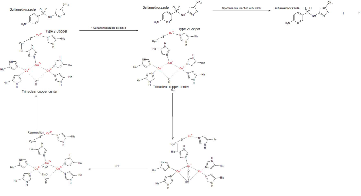
Figure 4. Picture of the reaction, showing how the enzyme acts on an arbitrary substrate. In this case, the substrate is SMX, the target substrate for our project. The histidines complexed around the copper are only for visual effect and more clarity on how they are conjugated within the enzyme. Also, several reaction steps involve the regeneration of $ Cu^{2+}$ in its oxidized form, including a peroxide intermediate. The charges set on the copper atoms are displaced within the metallocomplexes they are involved in.
Next, it is important to understand which parameters describe the actual reaction (regarding distances between functional groups, energies etc.), which conformations are productive binding modes, and which would not be active. In this case, bonds can be formed or broken, and we need to describe the very complex interactions of the SMX - copper complex. First of all, we need the self-consistent field calculations to converge to the lowest energy minima system, and not to any other, meaning the better we describe it, the more exact can we determine the system. Table 2 describes the HOMO-LUMO gap between different models, which will essentially be the driving force of the reaction (we will get back to this specific point).
Table 2. Shows HOMO-LUMO gap for different trials. A similar HOMO-LUMO gap in this case is correlated to which solution the method converged to. Similar HOMO-LUMO gaps meant similar orbital geometry.
| Scope of system | DFT functional | Basis set | HOMO-LUMO gap |
|---|---|---|---|
| Cu-centers, peripheral N atoms with methyl groups attached as well as SMX | B3LYP | 6-31G(d’,p’) | 15eV |
| Cu-centers, full peripheral histidine residues with SMX | B3LYP | 6-31G(d’,p’) | 0.1eV |
| Cu-centers, full peripheral histidine residues with SMX | B3LYP | cc-PVTZ | 0.12eV |
| Cu-centers, full peripheral histidine residues with SMX | PBE0 | 6-31G(d’,p’) | 0.1eV |
| Cu-centers, full peripheral histidine residues with SMX | XC-B3LYP | 6-31G(d’,p’) | 0.1eV |
| Cu-centers, full peripheral histidine residues with SMX | B3LYP | aug-ccPVTZ | never converged |
Given that the system was sufficiently described with correct orbital geometry in PBE0 - 631G compared to complex basis sets and the XC-B3LYP functional, it was sufficient to describe our system accurately. Moreover, the level of theory was used with TDDFT to show which electron was transferred from the substrate to the trinuclear copper center, and to determine the $\Delta G$ of the reaction. By then optimizing the charge separated triplet state the reorganizational energy could be arrived upon. We also found that for a number of different conformations of SMX in the binding pocket, the same result was arrived upon, meaning that as long as the substrate was close to the acceptor copper, the reaction could take place.
As described in the Integration and Analysis section, we also needed values of $\Delta G$ and $\lambda$ for another substrate for which the reaction could be tracked easier by absorbance difference over time, see the enzymatic assays page. This substrate was 2,2'-azino-bis(3-ethylbenzothiazoline-6-sulphonic acid), or ABTS. The same principle was used for this substrate, and the values for both substrates can be seen in Table 3. For the ABTS, the first excited state was not the charge transfer we were looking for as confirmed by Mulliken charge population analysis. Therefore, we chose the second state, which involved the charge transfer we were seeking, for root optimization (needed for finding $\lambda$).
Table 3. $\Delta G$ and the reorganizational energy of the system with SMX and ABTS.
| $\Delta G^o_{\mathrm{electron transfer}}$ [eV] | $\Delta \Delta G^o$ $state_{product} - state_{reactant}$ [eV] |
$\lambda$ (reorganizational energy) [eV] | |
|---|---|---|---|
| SMX | -1.4674 | -0.053924 | 1.4134752 |
| ABTS | -1.3802 | -0.06032 | 1.4091221 |
In the TDDFT results we only get a value of the energy, and across which orbitals the electron transfer happens. By visualizing the orbitals in Avogadro with an iso-value of 0.1, we can get a clearer view on how the electron transfer occurs. In the TDDFT calculation, the transfer of a single electron happened between several orbitals with several electrons, so that electrons from the SMX travel across the system with several miniscule transfers. They are shown below in Table 4. We can see that in the end, one extra electron was transferred to the acceptor orbital 365 than transferred from it. The orbitals are shown in Figure 5.
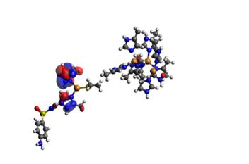
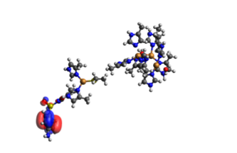
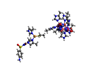
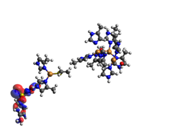
Figure 5.1. The donor orbitals for the full active site (the big cluster of atoms to the right) and SMX to the left of each individual picture.
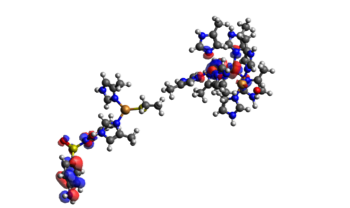
Figure 5.2. The main acceptor orbital (364) for the full active site (the big cluster of atoms to the right) and SMX to the left of each individual picture. This orbital is an antibonding orbital between SMX and the copper cluster.
Table 4. The electron transfers from different donor and acceptor groups in the complex.
| Donor | Acceptor | Energy difference |
|---|---|---|
| 353 | 364 | 0.12546 |
| 354 | 364 | 0.11448 |
| 355 | 364 | -0.24787 |
| 355 | 365 | -0.10251 |
| 356 | 364 | 0.59867 |
| 356 | 365 | 0.24769 |
| 364 | 356 | -0.24870 |
| 365 | 356 | -1.0278 |
The charge transfer was confirmed by Mulliken charge and population analysis in the QM routine, that showed a displacement of approximately 1 unit of negative charge from SMX to the active site. This had to be done since the acceptor orbital is not entirely localized on the active site, but there is a significant density present on the substrate as well. From this, we understood that the donor group (aminophenyl of the SMX) can be in many different conformations relative to the acceptor copper. For many systems, a linear correlation between the logarithm of electronic matrix coupling element and the distance between the donor and acceptor group can be seen. In our case, this means that the closer SMX gets to the copper upon binding to the binding pocket, the higher the $k_{cat}$ or $k_E$ can be, and the faster the reaction is.
It was at this point clear what had to be done - we would mutate the highly fluctuating phenylalanine residues at positions 162, 332 and 337 to smaller, less bulky residues that would simultaneously make the entropy contribution smaller, improving $K_M$, but also improving $k_cat$, by decreasing the distance between the SMX and the active site. We also saw that, except for some enthalpy contribution from pi-stacking, the hydrogen bond formed with aspartic acid at position 206 was crucial, which meant that if we could get the substrate closer to it, we would even get stronger bonding and thus lower $K_M$. This has also been shown before, in mutations from aspartic acid to glutamic acid that significantly lowered $K_M$ but also reduced $k_cat$ due to the distance getting higher.
Optimizing the System
First of all, for many mutations, we needed a systematic approach to test every mutation in the active site. One initial assumption was that, in order to use this supposed systematic approach for the system, the mutations could not affect the mechanism of electron transfer, nor induce too large changes in the folding of the protein.
Upon understanding the system better, it was determined that the distance between substrate and the acceptor copper had to be minimized, and the association optimized according to the equation $\Delta G = \Delta H - T \Delta S$. We then created a new model from this for specificity, stating that: $$ k_{ET(A > B)} = k * \left | V_{AB} \right |^2 e^{-\frac{(\Delta G-\lambda)^2}{4\lambda k_BT}} $$
... and that all conformations in productive binding modes have the same electronic distribution in the charge separated states (as shown before in Table 5), meaning that $\Delta G$ is constant for every conformation. The reorganizational energy is related to the slight change in geometry for the charge separated state. The assumption that was made was that the difference in reorganizational energy between binding modes would be negligible, i.e. distance-independant for productive binding modes (when the substrate binds sufficiently close). Reducing the distance-independent (but highly substrate dependent) terms to a constant $C$, we get:
$$ k_{ET}(d) = \left | V(d) \right |^2 * C_{\mathrm{substrate}} $$The V is, as previously mentioned, the geometric overlap of the orbitals. Since the electronic density around the center of the orbital decreases exponentially, we can get the shape of the function $\left | V(d) \right |^2$. Next, we used a similar approximation to simplify the distance dependence of the V(d) to the approximation used in: $$ k_{ET}(d) = 10^{13} * e^{-\beta d} * C_{\mathrm{substrate}} = Ae^{-\beta d} $$
Typically, $\beta = 1.4 \pm 0.2$ in proteins. However, this is based on the geometric overlap of the acceptor-donor orbitals assuming the electronic distribution lowers per unit of distance with $C e^{-\beta}$. The distance would then be the distance from the center of each orbital. In our case, we had to come up with a better equation for the geometric overlap, which we did by taking the geometric average of the two centers of the acceptor-donor orbitals. This distance could then be plotted across many conformations, giving us the $k_{ET}$ for each, which made us able to understand how fast the reaction would be catalyzed in a real, dynamic system. This is very contrary to the static approaches mostly seen in quantum mechanical calculations.
We could estimate the $k_{ET}$ with respect to the distance from the density center of the donor (SMX) to the density center of the acceptor (trinuclear copper cluster). To quickly be able to sample many conformations, we calculated the average specificity over the whole simulation for all of our mutants. This would hold true, given that the association energy does not fluctuate too much, making the $K_M$. Now that we had developed a method for testing different mutants, it was time to do so.
Firstly, however, the mutants had to be decided upon. Upon understanding that the dynamic system in the previous section, we figured that by removing the very volatile phenylalanine residues, although losing the enthalpy contribution to the interaction, we would also be able to get the substrate closer to the active site, which we now understand greatly increases the $k_{ET}$ of the reaction. With the time pressure of having to start testing experimentally the best-mutated candidate and obtain results on time, we decided to focus on mutating at positions 162, 332 and 337 from phenylalanine to less bulky residues. A major constraint to this method was that a similar fold had to be obtained in the simulation. Without a similar fold as the wild-type enzyme, the same reaction or similar $k_{ET}$ cannot be claimed, since the form may be inactive. The results can be found in the table below.
Video 1. Substrate sulfamethoxazole unable to stabilize the highly fluctuating phenylalanine residues of the laccase at positions 162, 332 and 337 - making it unable to enter the binding pocket of the laccase.
Video 2. Highly fluctuating phenylalanine residues of the laccase at position 162, 332 and 337 mutated to isoleucines. The SMX substrate is no longer stuck on the outside of the binding pocket. Instead it is able to enter the active site of the laccase, becoming a lot closer to the catalytic copper.
Table 5. The following table presents distance between substrate donor and active site acceptor orbital values from the MD simulations.
| Mutant | No. of frames | Average distance [Å] | Lowest distance [Å] | Highest distance [Å] |
|---|---|---|---|---|
| WILD TYPE | 1481 | 18.1985 | 24.6689 | 8.8845 |
| PHE162$\rightarrow$ILE162 PHE332$\rightarrow$ILE332 PHE337$\rightarrow$ILE337 |
3534 | 11.1260 | 17.8061 | 3.6393 |
| PHE162$\rightarrow$ALA162 PHE332$\rightarrow$ALA332 PHE337$\rightarrow$ALA337 |
3433 | 13.8381 | 23.9455 | 7.1623 |
| PHE162$\rightarrow$GLY162 PHE332$\rightarrow$GLY332 PHE337$\rightarrow$GLY337 |
3499 | 11.4159 | 20.1560 | 5.0026 |
At first sight, it seemed like the ILE and GLY substitutions were the most successful, however upon inspecting the simulations visually, we could see the reason for why all but the ILE substitution had very high maximum values of distance. Firstly, the wild-type seemed to dissociate mid-simulation, and only had about 1000 frames of the bound state (1 frame equals to 20 picoseconds, so every 50 frames is one nanosecond. 1000 frames is 500 ns). Secondly, the ALA and GLY substitutions misfolded during simulation. To illustrate this, we have included snapshots that show the misfolding of the active site in ALA and GLY, that can be seen in Figures 6-9 Therefore, the substrate dissociated quickly. A Molecular Dynamics simulation of the ILE-substitution mutant can is included in Video 2.
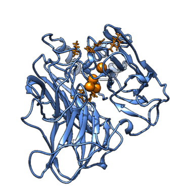
Figure 6. A snapshot of the Molecular Dynamics simulation with the substrate and the interesting mutated residues for the first mutant, with phenylalanine residues replaced by Isoleucine. It shows a similar active site structure to the wild type.
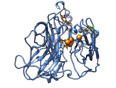
Figure 7. A snapshot of the Molecular Dynamics simulation with the substrate and the interesting mutated residues for the second mutant, with phenylalanine residues replaced by Alanine. It shows how the binding pocket has broadened, rendering it inactive (or at least we are not able to analyze it according to our method).
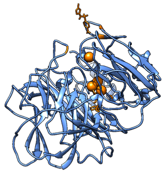
Figure 8. A snapshot of the Molecular Dynamics simulation with the substrate and the interesting mutated residues for the third mutant, with phenylalanine residues replaced by Glycine. It shows how the binding pocket has broadened, rendering it inactive (or at least we are not able to analyze it according to our method).
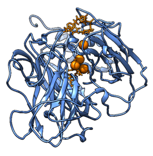
Figure 9. A snapshot of the Molecular Dynamics simulation with the substrate and the interesting residues for mutations of the wild type. It shows how the active site should look.
In addition, in Figure 10 and 11, you can see the distance in the $k_{cat}$ equation over the number of frames for the wild-type versus the ILE mutant. From these graphs, you can see how the substrate manages to stay closer to the active site of the ILE mutant rather than the wild type. It is also much more consistent in either being bound (in the start and end) or unbound state (in the middle) meaning less chance of being somewhere in between. We concluded that both $k_{cat}$ (thanks to distance) and $K_M$ could be improved. The theoretical values of $k_{cat}$ can be seen in Table 6.
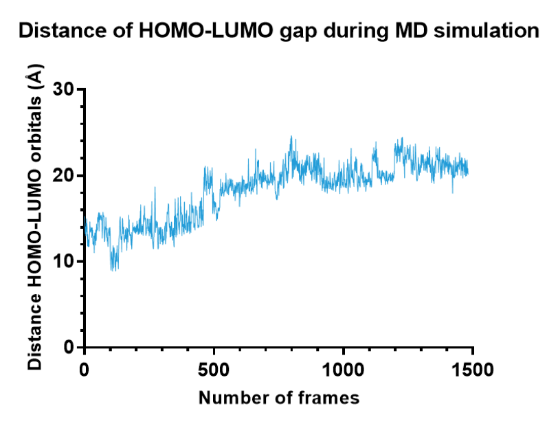
Figure 10. Distance between donor and acceptor orbitals in the wild-type over the whole MD simulation.
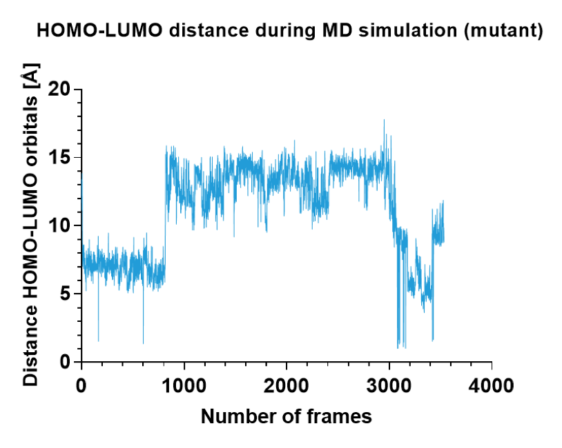
Figure 11. Distance between donor and acceptor orbitals in the successful ILE mutant over the whole MD simulation.
Table 6. Theoretical values of kcat for the mutated and wild-type laccases.
| System | $k_{cat,\mathrm{SMX}}$ (logarithmic average) | $k_{cat,\mathrm{SMX}}$ (linear $k_{cat}$ average) | $k_{cat,\mathrm{ABTS}}$ (logarithmic average) | $k_{cat,\mathrm{ABTS}}$ (linear $k_{cat}$ average) |
|---|---|---|---|---|
| Mutant theoretical (all frames) | 3.3277 $\mathrm{s}^{-\mathrm{1}}$ | 1297.2567 $\mathrm{s}^{-\mathrm{1}}$ | - | - |
| Mutant theoretical (only after equilibration) | 0.60544 $\mathrm{s}^{-\mathrm{1}}$ | 1121.5590 $\mathrm{s}^{-\mathrm{1}}$ | - | - |
| Mutant theoretical (only for frames when SMX is in the active site) | 249.19496 $\mathrm{s}^{-\mathrm{1}}$ | 56723.6185 $\mathrm{s}^{-\mathrm{1}}$ | - | - |
| WT theoretical (all frames) | 0.000163629 $\mathrm{s}^{-\mathrm{1}}$ | 0.4660223 $\mathrm{s}^{-\mathrm{1}}$ | ||
| WT theoretical (only after equilibration) | 0.10404 $\mathrm{s}^{-\mathrm{1}}$ | 1.661529 $\mathrm{s}^{-\mathrm{1}}$ | 0 $\mathrm{s}^{-\mathrm{1}}$ | 11.13041654 $\mathrm{s}^{-\mathrm{1}}$ |
| WT theoretical (only for frames when SMX is in the active site) | 0.10404 $\mathrm{s}^{-\mathrm{1}}$ | 1.661529 $\mathrm{s}^{-\mathrm{1}}$ | 0 $\mathrm{s}^{-\mathrm{1}}$ | 11.13041654 $\mathrm{s}^{-\mathrm{1}}$ |
References
- Jones, Stephen M.; Solomon, I. Edward. Electron transfer and reaction mechanism of laccases. Cell Mol Life Sci. 2015 Mar; 72(5): 869–883. Published online 2015 Jan 9. doi: 10.1007/s00018-014-1826-6
- Camarero, Susana; Pardo, Isabel. Laccase engineering by rational and evolutionary design. Cellular and Molecular Life Sciences, March 2015, Volume 72, Issue 5, 897-910 10.1007/s00018-014-1824-8
- Scheiblbrandner, Stefan; Breslmayr, Erik; Csarman, Florian; Paukner, Regina; Führer, Johannes; Herzog L. Peter; Shleev, Sergey V.; Osipov, Evgeny M.; Tikhonova, Tamara V.; Popov, Validimir O.; Haltrich, Dietmar; Ludwig, Roland; Kittl, Roman. Evolving stability and pH-dependent activity of the high redox potential Botrytis aclada laccase for enzymatic fuel cells. Scientific Reports 7, Article number 13688, 20 October 2017.
- Alcalde, Miguel; Mate M., Diana. Laccase engineering - from rational design to directed evolution. Biotechnology advances 33 (2015) 25-40. Elsevier.
- Dutta Dubey, Kshatresh; Shaik, Choreography of the Reductase and P450BM3 Domains Toward Electron Transfer Is Instigated by the Substrate. SasonJ. Am. Chem. Soc., 2018, 140 (2), pp 683–690. DOI: 10.1021/jacs.7b10072
Integration and Analysis
This section describes the results that we obtained experimentally in the lab and how we analyzed this data. In accordance with the rest of the modeling project, we inferred as much data as possible from the behavior of our laccase - how its properties change with pH, temperature and expression system. Throughout the extensive experimental part of the project, models were consulted to predict behavior that we would expect in the natural system. The success of these predictions could then be used to infer how our system actually works (or, as was the case most often, did not work).
Firstly, there were several steps where the computational and experimental parts integrated, and the interplay was mutual. Sometimes, a tidbit of information would pass in conversation and other times we would sit in long meetings to discuss data and how to progress. The interplay is visualized in the illustration below, showing which type of interaction it was and what information was exchanged (dry lab and wet lab refers to the computational and experimental work of our project respectively).
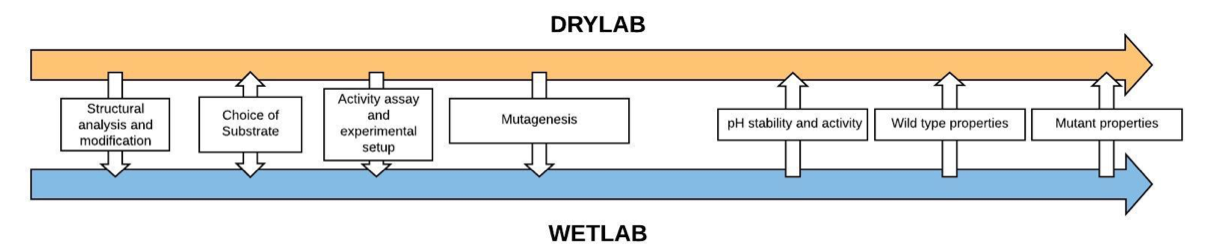
Figure 1. Visualisation of the model-experiment interplay during the iGEM Stockholm 2018 project. The arrows represent what information or interaction was exchanged and in what direction. Notice that the Choice of Substrate was a mutual exchange in both directions.
Structural Analysis and Modification
To be able to purify the enzyme we needed to add a purification tag. In our case, we chose the 6xHis-tag to be placed in one of the termini of the protein, since it has a high affinity towards an IMAC matrix, which we had available in the lab. However, adding 6 amino acids in the wrong terminus could be destructive for protein folding. Even though the gene sequence is linear, the encoded protein is not linear at all, folding into a complex three-dimensional structure. Upon structural analysis of the crystal structure 1GYC, we saw that the C-terminus was bending inward towards the active site, specifically to the trinuclear copper center. This suspicion was confirmed in MD, where the fold remained in the same conformation as observed in the crystal structure. For the N-terminus, we saw that it folded in an alpha-helix connected via at times 7 backbone hydrogen bonds to the surface of the protein. This looked as if it curled into the protein as well, but during MD we saw that it actually moved around to a much higher degree than expected. We thus decided to put the 6xHis-tag on the N-terminus of the protein, so as to not interfere with the active site.
Choice of Substrate
In a very early step during our project outline and development, we decided on SMX as our main target. One of the underlying reasons for this was that we needed to simultaneously find a substrate that, worked well with the chosen enzyme and fitted our goal - to make a difference and reduce ecotoxicity and antibiotic resistance in wastewater streams in the Baltic Sea region. After the team had come up with a series of substrates, we superposed each of them on a model substrate found in a similar crystal structure to see how well the chosen substrate fitted in the active site. One of the few that actually fitted neatly in the active site from the beginning was SMX. Some of the investigated substrates were trimethoprim, ciprofloxacin and tetracycline. All of these were significantly larger than SMX and were thus ejected during MD simulation.
Activity Assay and Experimental Setup
To be able to compare theoretical $k_{cat}$ and $K_M$ values with the experimentally obtained values, we needed to find a method that connected theory with reality. Since we are calculating energies, getting to measurable quantities such as $k_{cat}$ and $K_M$ should be done by the Arrhenius and Nernst equations respectively. In order for us to measure the correct parameters in the lab, we needed to understand how the reaction takes place, in which order, which rate determining step we have, or rather, under which conditions the most interesting step is the rate-determining step. The condensed reaction has the following major steps:
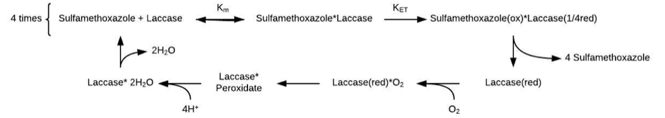
Figure 2. Condensed picture of the reaction. As shown, there are two major steps when only looking at what happens to the enzyme throughout the reaction - reduction at the top line, done by four SMX substrates separately, and then the bottom line that regenerates the laccase in its oxidized form, done by O2
As you can see in Figure 2, the reaction consists of several different steps. The only catalytic step involving the substrate is the kET, which is where the substrate is oxidized and the enzyme reduced (one-quarter of its full potential per substrate). When full, no more laccase can be oxidized and thus the reaction continues with regeneration. Due to the wildly different degradation times and kcat values of this enzyme for different substrates [1], we proposed that the electron transfer, the only substrate specific step, was the rate determining one. This means that the whole reaction can be condensed into:
$$ 4 \mathrm{SMX} + 4H^{+} + O_2 \rightarrow 4 \mathrm{SMX}^{\cdot+}+2H_2O $$This implies that the kinetics will involve SMX concentration, oxygen levels and pH. Thus, because we wanted to measure the kinetics of the first step in the reaction (electron transfer), we needed to make the other contributions as minimal as possible in the biochemical assays to faithfully determine the theoretical $K_M$ and $k_cat$ estimated via energies and electron transfer rates. This influenced the way the assays were planned out.
Mutagenesis
Mutagenesis comprised the bulk of the modeling project since the project revolved around developing a mutant laccase with higher activity than the original wild-type laccase for the chosen substrate (SMX).
In mutagenesis, we had to develop a new enzyme as described in the Methods and Results section, that had a higher affinity towards the chosen substrate. For this to work, we utilized MD, QM and QM/MM, and developed a new systematic approach to gauge the specificity $(\frac{k_{cat}}{K_M})$ of an enzyme to SMX (or for any substrate, given that new parameters for electron transfer and $K_M$ are calculated) for laccases and electron transfer reactions. This model was used to decide which mutant had the most potential for improving laccase specificity for SMX. In theory, this could be used for other systems of substrates and the laccase, that could improve the activity even further. This systematic approach to estimate the specificity was needed because only one set of mutations could be tested experimentally, due to limitations in time and resources.
Furthermore, the scope of the mutations was not allowed to be too large, since the mutations were originally planned to be integrated using site-directed mutagenesis in the lab. Because of this, too many mutations would make the process very time consuming and ineffective, so we were limited to mutations at about three sites, producing one final mutant. Although we ultimately chose to mutate three residues in the active site from phenylalanine to isoleucine, other strategies were proposed, as we will discuss in the Outlook page.
pH and Substrate
The first results gathered from the biochemical activity assays were on the pH and thermal stability of a similar commercial laccase from T. versicolor (38429 Sigma). Another substrate than SMX was used, namely 2,2'-azino-bis(3-ethylbenzothiazoline-6-sulphonic acid) (ABTS), because of the ease of following the reaction spectrophotometrically, as described in the enzymatic assay page. In the Methods and results section, it is outlined how the same reaction mechanism happens with ABTS as with SMX, only with different $k_{cat}$ and $K_M$. Their behavior under different conditions should, therefore, remain the same.
As expected, in the lab we saw a significantly higher $k_{cat}$ with a lower pH. However, while we did see a difference in $k_{cat}$ with lower pH, it was not as significant as we initially expected. To explain, the reaction looks like this:
$$ 4 \mathrm{SMX} + 4H^{+} + O_2 \rightarrow 4 \mathrm{SMX}^{\cdot+}+2H_2O $$Using only this reaction, we assume that the speed of the reaction is proportional, or at least slightly resembles $[H^+]^4$, which means that (in pH 4), $[H^+]$ is 1000 times higher than in pH 7, making the speed of the reaction supposedly 10^12, which would be way over the diffusion limit [2]. However, We did not see this drastic difference. As explained earlier, we supposed that the rate determining step would be SMX oxidation, as presented below: $$ SMX \rightarrow \mathrm{SMX}^{\cdot+} + e^{-} $$
Since the above-mentioned points were found in the lab, it was evident that the rate determining step was the electron transfer, as we already argued in the two previous sections. Because of this, we needed to find another explanation regarding why the activity is highest at about pH 4. Incidentally, we found a hydrogen bond between residue ASP206 (for which the $pK_a$ is 3.9 under standard conditions) and the residue at the NH2-group. This means that the association energy would be lower for the SMX/laccase complex, and we would get a higher thermodynamic driving force for the association, i.e. $K_M$ is lowered for the reaction, explaining the higher degradation rate.
Wild-Type Laccase Properties
In accordance with the modeling projects goals, we tried to gain as much understanding from small clues as possible, in order to get feedback to improve the models. Even though this was greatly limited by time, we were able to estimate $K_M$ and $k_{cat}$ values for the wild-type enzyme, since the $k_{cat}$ was a function of distance (see the Methods and Results section), a few averages were constructed for the wild-type, with respect to $k_{cat}$, log($k_cat$) and the average distance. The values of the average $k_{cat}$ can be seen in Table 1.
Table 1. Experimental values of $k_{cat}$ versus the theoretical values. SMX is Sulfamethoxazole and ABTS.
| System | $k_{\mathrm{cat},\mathrm{SMX}}$ (logarithmic average) | $k_{\mathrm{cat},\mathrm{SMX}}$ (linear $k_{cat}$) | $k_{\mathrm{cat},\mathrm{ABTS}}$ (logarithmic average) | $k_{\mathrm{cat},\mathrm{ABTS}}$ (linear average) | $k_{\mathrm{cat},\mathrm{ABTS}}$ (Michaelis- Menten assay) |
|---|---|---|---|---|---|
| WT theoretical (all frames) | 0.000163629 $s{-1}$ | 0.4660223 $s{-1}$ | 0 $s{-1}$ | 4.901903262 $s{-1}$ | - |
| WT theoretical (only after equilibration) | 0,10404 $s{-1}$ | 1,661529 $s{-1}$ | 0 $s{-1}$ | 11,13041654 $s{-1}$ | - |
| Experimental WT | - | - | - | - | 4.2 $s^{-1}$ |
During association in the MD simulation, no significant change in total energy occurred as the substrate bound to the binding pocket, which was why we deemed that the $\frac{K_M}{K_D}$ approximation was valid. As seen in Figure 3 below, few steric groups seem to clash with SMX on its way out or into the binding pocket, making the transitional energy $\Delta G^{T}$ lower. We deemed this to be higher than the very low k_{cat} values that we both calculated and arrived at experimentally.
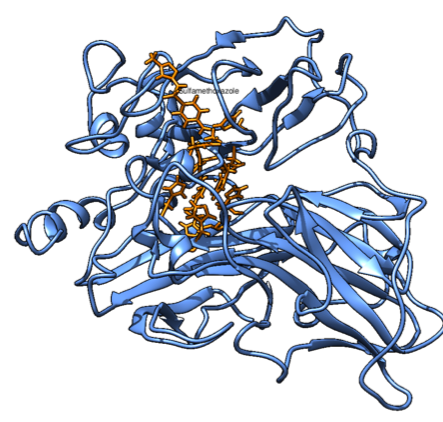
Figure 3. The graphic shows what happened during the MD simulation as the substrate bound to the binding pocket.
The linear average of $k_{cat}$ is always higher than the logarithmic average value, as some conformations are simply too far from the active site, and will dominate the logarithmic average. We suppose that the linear average is a better representation of $k_{cat}$ since the conformations with largest $k_{cat}$ will dominate the average. We think this represents what you would find in reality, since the largest $k_{cat}$ conformations will catalyze much more substrate and will dominate conformations that do not have the same catalytic ability. While both SMX and ABTS had similar energetic values, the HOMO-LUMO gap was smaller for ABTS, since the donor orbital gets closer to the active site than what the donor orbital of SMX can. This geometry seems to be the reason as for why ABTS reacts faster. The similar energetic values ($\Delta G$ and reorganizational energy) are probably due to that the redox potential of the laccase dominates the thermodynamics of the reaction. The $k_{cat}$ from the enzymatic assays was very close to the linear average of $k_{cat}$, giving evidence that this approach can be used for substrates of this laccase.
From this, we could draw the conclusion that the modeling of the reaction actually exceeded our expectations regarding accuracy. In addition, we knew that we could use the approximation of $k_{cat}$ being dependant on distance for productive binding modes. The same could then be compared with the mutants, given that the assumptions leading up to the model could be justified. Sadly, they were not.
Mutant Properties
For the mutant, a higher $k_{cat}$ and similar $K_M$ were estimated through the same procedure as for the wild type. The results of this simulation can be seen in Table 2.
Table 1. Experimental values of $k_{cat}$ versus the theoretical values. SMX is sulfamethoxazole and ABTS.
| System | $k_{cat}$ (distance average) | $k_{cat}$ (logarithmic average) | $k_{cat}$ (linear $k_{cat}$ average) |
|---|---|---|---|
| Mutant theoretical (all frames) | 3.3277 $s^{-1}$ | 3.3277 $s^{-1}$ | 1297.2567 $s^{-1}$ |
| Mutant theoretical (only after equilibration) | 0.60544 $s^{-1}$ | 0,60544 $s^{-1}$ | 1121.5590 $s^{-1}$ |
| Mutant theoretical (only for frames when SMX is in the active site) | 249.19496 $s^{-1}$ | 249.19496 $s^{-1}$ | 56723.6185 $s^{-1}$ |
Even though the same strategy was used for the production of the mutant as for the wild-type laccase, the mutant failed to be expressed several times. A plethora of things could have gone wrong during both experimental and modeling procedures; however, from colony PCR we knew that the genetic construct had been integrated into the genome of our host. Since the SDS-page results were inconclusive, we also could not say that a protein of our size existed. For more information, see the Laccase production page. In short, even though the gene was present, we could not measure the activity of the enzyme. Because of the very accurate $k_{cat}$ estimation in the previous section, we considered that the methodology of the modeling was not faulty, but that we had encountered a system that did not abide by the assumptions we had set up for the system. The most significant of these, as described in the Methods and results section was that the mutant would not fold in the same way as the wild-type. To try to explain the behavior of the mutant, another MD simulation was run with slightly higher temperature, setting $T_0=310K$, to see if there were other folding modes that we missed during the first MD simulations of the mutants.
The results of this run can be seen in Figure 4. There was clearly an alternative fold, similar to the spreading seen in the runs with significantly smaller residues. A contributing reason to why we did not see this effect in the original MD simulation was that the substrate was too tightly bound for water molecules or the tension in the protein to take effect and unfold the binding pocket. This could be a valid explanation for the misbehavior of the mutant laccase. In the methods and results section, we actually saw hints of the behavior evident in Figure 4. We see that there is some tension in the backbone of the protein, forcing it open if there are no stabilizing residues to stop it. This “hinge-structure” is probably a second folding mode, that we discovered by increasing the temperature a bit. This raised the speed with which the enzyme decayed to a state with lower energy, to which the thermodynamic driving forces point.
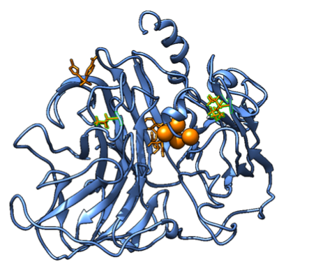
Figure 4. A graphic showing the protein unfolding slowly during the temperature increase, leaving the substrate unbound and an inactive protein, since SMX will not bind close to the active site specifically. The mutated residues are highlighted with a green outline, while the big spheres are the coppers in the active site. A small organic molecule to the left is SMX, that is completely dissociated.
In addition, we can look at the radius of gyration of the protein only, disregarding the solvent, by using the radgyr command in the cpptraj subroutine of the ambertools suite to confirm that it does indeed increase over the course of this simulation. As shown in Figure 5, a clear upwards trend is present, which confirms the visual clue that suggested an unwrapping or unfolding of the protein.
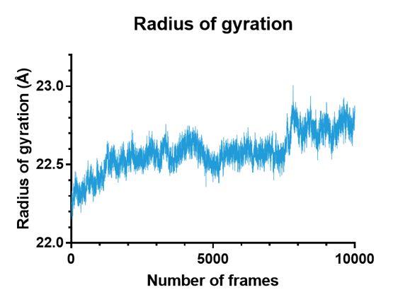
Figure 5. Radius of gyration plotted against the number of frames of the simulation for the mutant at a higher temperature $T_0=310K$, showing an upwards trend.
This analysis is crucial for the next generation, where we would aim to improve the laccase even further, given that we know even more dynamic parameters of the system now. From the mutant, we can say that we removed important $\pi$-$\pi$ interactions between the phenyl alanine residues, which released the tension across the binding pocket and unfolded it. This is to be discussed further in the outlook page. The modeled $k_{cat}$ for the mutant, however, was reported to be about 300 times higher than the experimental $k_{cat}$ of the wild type, showing that if the mutant would have folded properly, we would have likely had significantly higher $k_{cat}$-values.
References
- Jones, Stephen M.; Solomon, I. Edward. Electron transfer and reaction mechanism of laccases. Cell Mol Life Sci. 2015 Mar; 72(5): 869–883. Published online 2015 Jan 9. doi: 10.1007/s00018-014-1826-6
- Sean A. Fischer, Brett I. Dunlap, Daniel Gunlycke. Correlated Dynamics in Aqueous Proton Diffusion, 13 march 2018. Physics-chem-ph