Team:Leiden/Model
Model
In science, crafting theoretical models can help understand, predict and improve experiments and their interpretation. In our project, theoretical modelling was used to optimise the experimental setup for the Read more about our optimized experimental setup on the Results page validation of our stress-responsive chromoprotein strains on agar. For this purpose, we created a diffusion
model of
antibiotics through agar in disk diffusion.
In the background section, more information about disk diffusion and how this relates to our project will be provided. In addition, two different diffusion models will be evaluated through a series of experiments. In the next two sections, a
linear 1-dimensional diffusion model is created and validated with strains that express GFP and chromoproteins respectively in response to stress. The final section is a 2-dimensional diffusion model to further optimise the experimental
setup
for disk diffusion with chromoprotein strains.
After speaking with Read more about our interview with prof. Van Wezel on our Integrated Human Practices page
prof.
Gilles
van Wezel about the applications of our stress response system, we developed a strain that produces chromoproteins - visible to the naked eye - when exposed to stress. This way, our detection system could be used in Streptomyces
overlays: experiments in which potential antibiotic producing strains are grown on a plate, after which a bacterial test strain is seeded on top. Compounds diffuse through the agar and - if lethal - prevent bacterial growth, thereby
creating a “zone of inhibition" around the Streptomyces strains[1].
For the use of chromoproteins in these experiments, an understanding of the dose response of chromoprotein production and the consequences for chromoprotein visibility on agar is necessary. Therefore, we decided to model the diffusion of
the antibiotic nalidixic acid through agar during a disk diffusion assay, in order to understand the distribution of nalidixic acid concentration, and therefore the resulting chromoprotein stress response.
To assess whether the chromoproteins would be visible on agar after exposure to stress, we started with a more controlled setup compared to Streptomyces overlays, known as disk diffusion. Disk diffusion assays are used in antibiotic
susceptibility testing and are simple experiments where - instead of growing Streptomyces - disks containing antibiotics are placed on an agar layer with growing bacteria[1].
Theoretical Model
The interpretation of disk diffusion assays is usually performed using a model-dependent analysis. Both the minimum inhibitory concentration (MIC value) and the diffusion constant of the compound in question can be estimated from a series of experiments using diffusion models. Often, the diffusion of the compound is modelled as free, linear diffusion using Fick's second law: $$ \frac{\partial c}{\partial t} = D \frac{\partial^2 c}{\partial x^2} $$ From this equation, the following relation between the diffusion constant ($ D $), MIC value and concentration can be derived: $$ \ln(\text{MIC}) = \ln(c) - \frac{x^2}{4Dt} $$ This approximation has been applied successfully to diffusion studies of a number of antibiotics, such as penicillin and nisin[2,3]. However, certain hydrophobic or amphiphilic compounds cause zones of inhibitions that scale linearly rather than quadratic with concentration. To account for this, Bonev et al. proposed a different model, which is essentially a modification on Fick's law[4]. By adding a dissipative term describing the loss of antibiotic as it moves through the agar, the concentration over time becomes: $$ \frac{\partial c}{\partial t} = D\frac{\partial^2 c}{\partial x^2} + V\frac{\partial c}{\partial x}$$ This equation yields the following relationship between the diameter of the zone of inhibition and the concentration $ \ln(c) $: $$ \ln(\text{MIC}) = \ln(c) - \frac{x^2}{4Dt} $$
Experimental Validation
To evaluate which approximation was more suitable for developing a diffusion model, a series of disk diffusion assays was performed with nalidixic acid and E. coli Dh5α. The initial concentration of nalidixic acid in the disks was varied from 0.05 μg/mL to 50 μg/mL, and the resulting size of the zone of inhibition was measured after 24 hours using ImageJ. Then, the diameter of this zone ($ x $) was plotted against the natural logarithm of the concentration of nalidixic acid ($ \ln(c) $) according to both models. Linear regression was used to determine the best linear fit (see Figure 1).
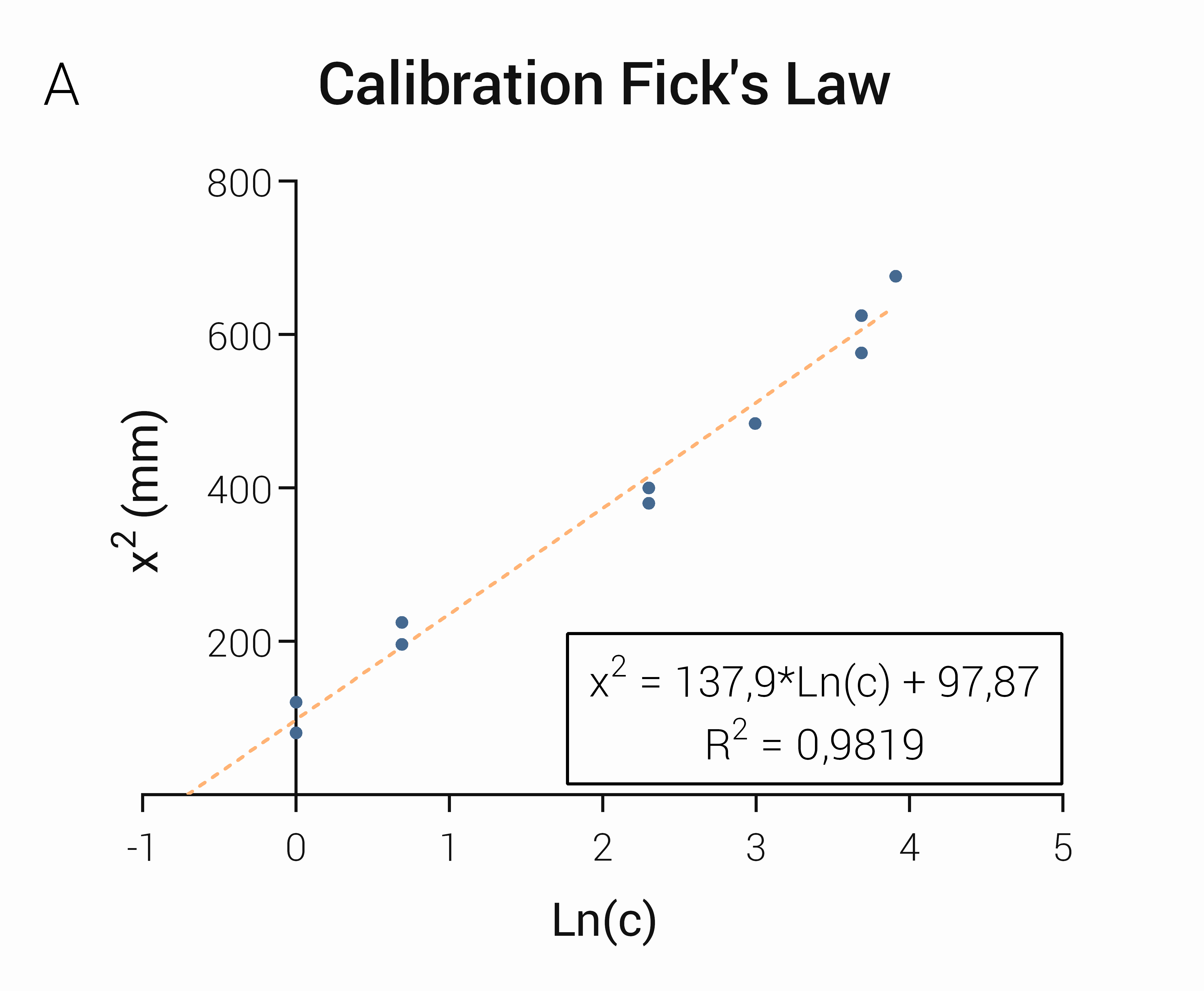

The R2-value for the original Fick's second law is higher than compared to Bonev's modification, indicating a better fit to that model (Figure 1). Using the linear fit to Fick's second law, we then calculated the apparent diffusion constant of nalidixic acid in agar. This diffusion constant of 1.347 mm/hour was then used when modelling the diffusion over time.
Conclusion
For bacterial overlays, more information about the visibility and responsiveness of chromoprotein expressing strains is key. We therefore decided to model the diffusion of nalidixic acid. For this, we evaluated 2 diffusion models and experimentally determined that a model using Fick's second law would be most suitable for our diffusion model.
References
[1]: Balouiri M., Sadiki M., Ibnsouda SK. Methods for n vitro evaluating antimicrobial activity: A review. Journal of Pharmaceutical Analysis (2015), 6(2), 71-79
[2]: Chandrasekar V, Knabel SJ, Anantheswaran RC. Modeling development of inhibition zones in an agar diffusion bioassay. Food Science & Nutrition (2015), 3(5), 394-403
[3]: Cooper KE, Woodman D. The diffusion of antiseptics through agar gels, with special reference to the agar cup assay method of estimating the activity of penicillin, J Pathol Bacteriol (1946), 58, 75-84
[4]: Bonev B., Hooper J., Parisot J. (2008) Principles of assessing bacterial susceptibility to antibiotics using the agar diffusion method, Journal of Antimicrobial Chemotherapy, 61(8), 1295–1301
After experimental determination of the diffusion coefficient, we used Fick's second law to create a linear 1D diffusion model and modelled the nalidixic acid concentration in agar over time. These predicted concentrations were then validated with our pSoxS-GFP-pSsoxS-GFP biobrick (BBa_K2610034) using confocal microscopy.
Theoretical Model
To solve the ordinary differential equation given by Fick's law, we use a finite difference approach known as the Forward Euler method. For this, we must first define the initial and boundary conditions. The initial condition is the concentration profile at the start of the experiments and is represented by function $I(x)$: $$ u(x,0) = I(x), \quad x\in [0,L] $$ As boundary conditions, the concentration at the edges of the petri dish were assumed to be 0 at all times: $$ u(0,t) = 0, \quad t>0 $$ $$ u(w,t) = 0, \quad t>0 $$ Then, the width of a petri dish and the time (domain $ [0,w]$×$[0,T] $ ) were both approximated by a series of mesh points: $$ x_i=i\Delta x $$ $$ T_i=i\Delta T $$ Lastly, the derivatives were approximated by linear combinations of function values at the grid point using a forward difference in time and a central difference in space: $$ \frac{u^{n+1}_i-u^n_i}{\Delta t} = D \frac{u^{n}_{i+1} - 2u^n_i + u^n_{i-1}}{\Delta x^2} $$ This was all modelled using Python 3.6 for which all the code can be found in the appendix.
Experimental Validation
Before starting experiments with chromoprotein expressing constructs, we validated this diffusion model with a GFP expressing strain. The pSoxS-GFP-pSoxS-GFP (BBa_K2610034) construct in E. coli, which showed the highest GFP expression in response to nalidixic acid in Read more about the GFP expression of this construct on our Results page. flow cytometry measurements, was used as the indicator strain in disk diffusion with a single disk with 10 μg/mL nalidixic acid. After 24 hours of incubation, GFP expression of bacteria that were growing 20 mm from the centre of the disk was compared to bacteria 45 mm from the centre of the disk using confocal microscopy (Figure 3).

As seen in the above figure, bacteria growing 20 mm from the centre of the disk show a higher GFP expression than bacteria growing further away from the disks. This suggests that a concentration profile of a stress-inducing compound can be detected with GFP-expressing strains.
Conclusion
In this chapter, a linear 1-dimensional free diffusion model was created according to Fick’s second law. The concentration gradient of nalidixic acid and its effect on a GFP expressing reporter strain (pSoxS-GFP-pSoxS-GFP, BBa_K2610034) was then measured to successfully validate this model.
After successfully validating our 1D diffusion model with the GFP pSoxS-GFP-pSoxS-GFP (BBa_K2610034) strain in combination with nalidixic acid, we started experiments with the pSoxS-AmilCP (blue chromoprotein) (BBa_K2610033) strain. To increase the visibility we explored the creation of a "stress zone" with our 1D model.
Theoretical Model
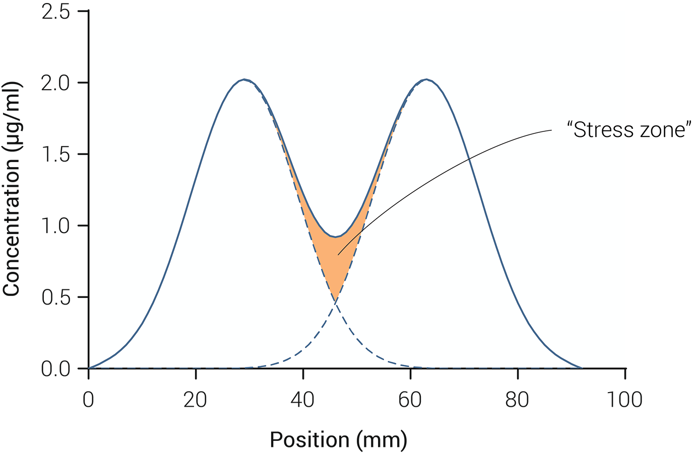
Using the same 1D free diffusion model from the previous section, the system was expanded to two disks with nalidixic acid and modelled over a time period of 48 hours. After 12 hours, the concentration profile of nalidixic acid between the two disks starts to overlap, creating a "stress zone" (Figure 4 and 5).
Experimental Validation
Using the stress zone principle from the 1D model described above, we performed a disk diffusion experiment with 3 disks placed in a triangle and a (blue) chromoprotein expressing strain pSoxS-AmilCP (BBa_K2610033). The triangle shape was used to increase the surface area of the stress zone. The initial concentration of nalidixic acid in the disks was 10 μg/mL. After 48 hours, a small blue-ish halo appeared around the zone of inhibition which validated our pSoxS-AmilCP (BBa_K2610033) strain (Figure 6).
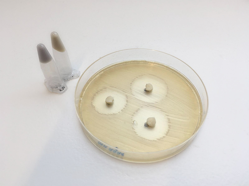
It must be noted that no stress zone between the three disks was visible in these experiments as only a small area around the zone of inhibition showed a change in colour.
Conclusion
In this chapter, we expanded our 1-dimensional diffusion model to multiple disks and saw that the concentration profiles of nalidixic acid can overlap and theoretically create a zone of stress. We experimentally validated our pSoxS-AmilCP strain (BBa_K2610033), which showed a beautiful blue halo around the zone of inhibition although no "stress zone" could be detected.
After successfully using our theoretical approach to validate the response of our pSoxS-AmilCP (BBa_K2610033) to nalidixic acid, we created a 2D model to obtain more detailed information about the nalidixic acid concentrations in the petri dish.
Theoretical Model
Whilst the 1D diffusion model predicted a concentration profile and the appearance of stress zones, disk diffusion experiments showed that pSoxS-AmilCP (BBa_K2610033) only showed a visible reaction around the edges of the zone of inhibition. To help understand the response of pSoxS-AmilCP (BBa_K2610033) showing a change in colour, we expanded the diffusion model to 2 dimensions. This would allow for a better estimation of nalidixic acid in the agar at that location. In two dimensions, Fick's second law becomes: $$ \frac{\partial c}{\partial t}=D \bigg( \frac{\partial^2 c}{\partial x^2} + \frac{\partial^2 c}{\partial y^2} \bigg) $$ Similarly to the 1D model, the Forward Euler finite difference approach was used to model the 2D diffusion over time. The petri dish was modelled as a 92 × 92 mm square grid and the three disks were modelled as circles with a uniform initial concentration. In terms of boundary conditions, the concentration of nalidixic acid at the edges of the petri dish was again assumed to be zero. Taking those initial and boundary conditions, the space and time domain were again discretized and the function was approximated using a forward difference in time and a central difference in space: $$ \frac{u_{i,j}^{(n+1)} - u_{i,j}^{(n)}}{\Delta t} = D\left[ \frac{u_{i+1,j}^{(n)} - 2u_{i,j}^{(n)} + u_{i-1,j}^{(n)}}{(\Delta x)^2} + \frac{u_{i,j+1}^{(n)} - 2u_{i,j}^{(n)} + u_{i,j-1}^{(n)}}{(\Delta y)^2} \right] $$ Using this method, the concentration profile was modelled over a time period of 48 hours (Figure 7).
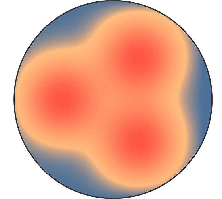
To (visually) compare these results to the GFP strains that had been tested more in depth with flow cytometry and confocal microscopy, we showed the "minimal stressful concentration" of nalidixic acid in pSoxS-GFP (BBa_K2610031) in orange (Figure 7 and 8). After 48 hours, it can be seen that the nalidixic acid concentration in the petri dish has reached "stressful" levels almost everywhere. This is interesting as this shows a clear difference in (visible) dose response between the pSoxS-AmilCP (BBa_K2610033) and pSoxS-GFP strains.
Experimental Validation
To further evaluate the dose response of pSoxS-AmilCP (BBa_K2610033), we started serial dilution experiments. These are liquid culture experiments, in which the concentration of nalidixic acid is varied, allowing for an easy read-out of any difference in AmilCP expression. Although Read more about the liquid culture experiments with AmilCP on our Results page. these experiments did not yield a clear answer for the discrepancy between the diffusion model and the performed disk diffusion experiment (Figure 6), it was noted that the expression of AmilCP needs at least 24 hours before a blue colour is visible. This could be the reason that only a small halo is blue and not the entire plate, as the model suggests that only after 48 hours the entire plate has a stressful concentration.
Conclusion
In this chapter, a 2-dimensional diffusion model was created to understand the dose response of pSoxS-AmilCP (BBa_K2610033). After modelling the nalidixic acid in the petri dish over 48 hours and comparing expression of chromoproteins to flow cytometry experiments with pSoxS-GFP, we concluded that the dose response of pSoxS-AmilCP (BBa_K2610033) is different, likely due to the time needed for the AmilCP to reach high enough concentrations in the cells to be visible to the naked eye.
Assumptions
- Several assumptions were made when modelling the diffusion of nalidixic acid over time:
- Only mass transport through diffusion, convection was neglected
- Diffusion was possible through a semi-solid medium, without loss of antibiotic through reaction
- The agar was uniform in concentration
- The concentration of nalidixic acid at the start was uniform in the disks
Python codes
1D diffusion:
          """

          Simple 1D diffusion model for disk diffusion/Kirby Bauer by iGEM Leiden 2018

          """

          import numpy as np

          import matplotlib.pyplot as plt

          """

          Defining basic parameters

          """

          W = 92 # Plate size, mm

          Nx = 92 # Number of 'steps' in space

          D = 2 # Diffusion constant antibiotic in agar, mm2 hour-1

          dt = 0 # Time step, hours

          Nt = 1000 # Number of timesteps

          F = 0.3

          T = 49

          """

          Initial concentrations antibiotic in petridish and on disk

          """

          Ca1 = 10 # Concentration antibiotic on disk 1, ug/ml

          Ca2 = 10 # Concentration antibiotic on disk 2, ug/ml

          Ca0 = 0 # Concentration antibiotic in petridish, ug/ml

          def I(x):

          #if x > 26 and x < 32:

            # return Ca1

            if x> 60 and x < 66:

              return Ca2

              else: return Ca0

              """

              Diffusion in 1D calculation, with forward-difference in time and central-difference in space

              “""

              def solver_FE_simple(I, D, W, Nx, F, T):

              x = np.linspace(0, W, Nx+1) # mesh points in space

              dx = x[1] - x[0]

              dt = F*dx**2/D

              timestamps = [24]

              for T in timestamps:

              u_1 = np.zeros(Nx+1)

              for i in range(0, Nx+1):

              u_1[i] = I(x[i])

              Nt = int(round(T/float(dt)))

              t = np.linspace(0, T, Nt+1) # mesh points in time

              u = np.zeros(Nx+1)

              for n in range(0, Nt):

              for i in range(1, Nx):

              u[i] = u_1[i] + F*(u_1[i-1] - 2*u_1[i] + u_1[i+1])

              u[0] = 0; u[Nx] = 0 # Insert boundary conditions

              u_1, u = u, u_1


              plt.plot(x,u)


              return u


              """

              Output --> Csv file

              """


              data = solver_FE_simple(I, D, W, Nx, F, T)

              print(data)

              np.savetxt("1dmodeltest.csv", data, fmt= '%1.4e', delimiter=',')
2D diffusion:
          """

          Simple 2D diffusion model for disk diffusion/Kirby Bauer by iGEM Leiden 2018

          """

          import numpy as np

          """

          Defining basic parameters

          """

          w = h = 120 # Plate size, mm

          D = 1.437 # Diffusion constant antibiotic in agar, mm2 hour-1

          dx = dy = 1

          nsteps = 300 # Number of timesteps

          dt = (dx**2)/(4*D)

          nx, ny = int(w/dx), int(h/dy)

          dx2 = dx*dx

          dy2 = dy*dy

          """

          Initial concentrations antibiotic in petri dish and on disk

          """

          C0 = 0 # Concentration antibiotic in petri dish, ug/ml

          Ca = 10 # Concentration antibiotic on disk, ug/ml

          r = 3 # Radius disks, mm

          disk_x1 = 20 # location disk 1, mm

          disk_y1 = 25 # location disk 1, mm


          disk_x2 = 20 # location disk 2, mm

          disk_y2 = 60 # location disk 2, mm


          disk_x3 = 20 # location disk 3, mm

          disk_y3 = 95 # location disk 3, mm


          uchan = C0 * np.ones((nx, ny))

          u = np.zeros((nx, ny))


          r1 = r**2

          for i in range(ny):

          for j in range(nx):

          p2 = (i*dx-disk_x1)**2 + (j*dy-disk_y1)**2

          if p2 < r1:
uchan[i,j]=Ca

for i in range(ny):
for j in range(nx):
p2=(i*dx-disk_x2)**2 + (j*dy-disk_y2)**2
if p2 < r1:
uchan[i,j]=Ca

for i in range(ny):
for j in range(nx):

              p2=(i*dx-disk_x3)**2
              + (j*dy-disk_y3)**2
if p2 < r1:
uchan[i,j]=Ca


                """

                Diffusion in 2D calculation, with forward-difference in time and central-difference in space

                """
def do_timestep(uchan, u):
u[1:-1, 1:-1]=uchan[1:-1, 1:-1] + D * dt * (
(uchan[2:, 1:-1] - 2*uchan[1:-1, 1:-1] + uchan[:-2, 1:-1])/dx2 +
                (uchan[1:-1, 2:] - 2*uchan[1:-1, 1:-1] + uchan[1:-1, :-2])/dy2
 )

uchan=u.copy()
return uchan, u
 x_values=np.linspace(0,w,nx)

 """

                Output --> Csv file

                """

                time=[276] # Define point in time for output
# Output csv file with data
for m in
                range(nsteps):
uchan, u=do_timestep(uchan, u)
if m in time:
 met_x=np.vstack([x_values,u])
print(u)
np.savetxt('2dmodeltestwikit48.csv', met_x, fmt='%1.6e' , delimiter=',' )