Team:St Andrews/Model

Modelling

⤵

• Introduction
• Cell Lysis Model
• Biofilm Model
• References

Introduction

The model is written in differential equations, which describe the rate of change for something in terms of a function. In our case the 'thing' changing is concentration of a protein and our equation is a function of time. This is notated as \(\frac{dA}{dt}\) where A is a function describing the concentration of a protein and t is time. A positive \(\frac{dA}{dt}\) denotes increase in our thing A with time, and a negative \(\frac{dA}{dt}\) denotes a decrease in A with time. Similarly, \(\frac{dA}{dt}=0\) denotes no increase or decrease in the amount of \(A\) over time and is thus called a steady state of A. We use this description of the system to study the system's behaviour.

How are we studying the model? There are algorithms which one can use to approximate the value of a function at a point based on the differential equation for that function, i.e. for the general differential equation \(\frac{dy}{dx} = f(x)\) , we can approximate \(y(x)\) using \(f(x)\) and a known initial value. There are a few algorithms which achieve this to varying degrees of accuracy, but the algorithms we're using are called Runge-Kutta methods. We use Python to implement these and use the python library matplotlib to visualise the functions.

Cell lysis model

For the purposes of the model, we consider the concentrations of the protein components as functions of time: \([mNG_{11}](t)\), \( [mNG_{1-10}](t)\), and \([mNG](t)\). The functions represent the extracellular concentrations of these proteins at a point in space. The position of these points in space affects the model. The point can either be within the lysed \(mNG_{1-10}\) expressing cell or in a point at extracellular space. We assume that the \(mNG_{11}\) expressing cell lyses with the \(mNG_{1-10}\) cell, and that \([mNG]=0\) at \(t=0\). This yields two cases:

Case 1 – Point within lysed \(mNG_{1-10}\) cell

In this case we treat the \(mNG_{1-10}\) as released solely at one point in space, with entry of \(mNG_{11}\) from outside the cell to the point being the rate-limiting factor. We describe this system as follows:

\begin{align} &\frac{d[mNG_{11}]}{dt} = \frac{\beta x^2}{x^2 + t^2} - \theta [mNG_{11}][mNG_{1-10}]\\ &\frac{d[mNG_{1-10}]}{dt} = - \theta[mNG_{11}][mNG_{1-10}]\\ &\frac{d[mNG]}{dt} = \theta [mNG_{11}][mNG_{1-10}]-\mu[mNG] \end{align}

Where \(\theta\) represents the rate constant for the forward reaction \(mNG_{1-10} + mNG_{11} \longrightarrow mNG\), \(\mu\) represents the loss of fluorescent \(mNG\) to photobleaching. As we assume all the \(mNG_{1-10}\) in our system is released at a point, there is no input of \(mNG_{1-10}\) in equation 2 and \(mNG_{1-10}\) is removed at the rate of the forward reaction. \(mNG_{11}\) is assumed to enter the point via diffusion and the \(\frac{\beta x^2}{x^2 + t^2}\) term describes this. Here \(\beta\) is the rate of \(mNG_{11}\) input at \(t=0\), and the constant \(x\) controls how quickly the term decreases to \(0\) as \(t \rightarrow \infty\). This decreases to \(0\) with \(t\) as we expect the system to reach an equilibrium with time where \([mNG_{11}]\) remains constant, either due to all \(mNG_{11}\) molecules assembling to an \(mNG\) or constant concentration in the surrounding area of our point, i.e. diffusion into the point being equal to diffusion out.

A term of the form \(\frac{\beta x^2}{x^2 + t^2}\) was chosen following a conversation with Dr Chris Hooley, who pointed out to us a term such as \(\frac{\beta}{t}\) tends to \(0\) but integrates to \(\beta ln(t)\), a function with no bound as \(t \rightarrow \infty\), i.e. an infinite concentration of \(mNG_{11}\)! An also more glaring issue is discontinuity of the function at \(t=0\), hence why we did not select a term of the form \(\frac{\beta}{t^2}\), which would imply infinite rate of \(mNG_{11}\) input as \(t \rightarrow 0\).

By inspection, one can find that the steady state of this system (where \(\frac{d[mNG_{11}]}{dt} = \frac{d[mNG_{1-10}]}{dt} = \frac{d[mNG]}{dt} =0\)) occurs at \(t=\infty\) where \([mNG]=[mNG_{1-10}]=0\) or \([mNG]=[mNG_{11}]=0\).

Point out-with lysed \(mNG_{1-10}\) expressing cell

Here we treat a point in space outside the lysed \(mNG_{1-10}\) cell, where \(mNG_{1-10}\) and \(mNG_{11}\) enter via diffusion. Whilst we can assume here \(mNG_{11}\) is present in excess, we need to model its replenishment after reaction and hence include an input term analogous to the one in equation 1. The model for this system is as follows:

\begin{align} &\frac{d[mNG_{11}]}{dt} = \frac{\beta x^2}{x^2 + t^2} - \theta [mNG_{11}][mNG_{1-10}]\\ &\frac{d[mNG_{1-10}]}{dt} = \frac{\epsilon \tau^2}{\tau^2 + t^2} - \theta [mNG_{11}][mNG_{1-10}]\\ &\frac{d[mNG]}{dt} = \theta [mNG_{11}][mNG_{1-10}]-\mu[mNG] \end{align}

\(\tau\) and \(\epsilon\) are analogous to the \(x\) and \(\beta\) terms in equation 1. \(\mu\) and \(\theta\) are defined to be the same constants as in case 1.

This has a steady state, at \(t=\infty\) where \([mNG_{1-10}]=0\) and \([mNG]=0\).

Model Parameters

Below is a table with values for the model constants.

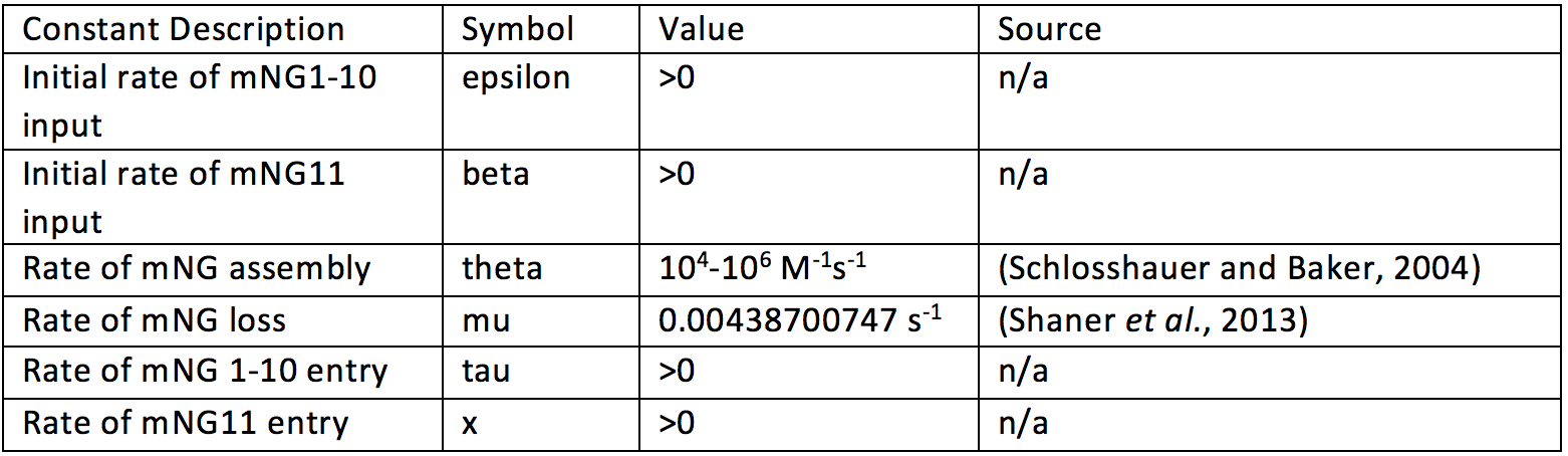
Unfortunately some constants could not be determined from experiment or literature. These are input constants.

The initial values of \([mNG_{11}](t)\) and \([mNG_{1-10}](t)\) could not be determined (or approximated) based off of promoter strength as we do not know how long the cells have been expressing \(mNG_{11}\) and \(mNG_{1-10}\) for.

Model Behaviour

As not all the constants have been resolved for our system, we can only guess suitable values when studying model behaviour.

Figure 1 shows the behaviour of the Case 1 model over time, for some guess constants. These were chosen as they serve to illustrate the predicted behaviour of the system based on biological intuition. It shows the key behaviours: \([mNG](t)\) tending to a steady limit over time, decrease of \([mNG_{1-10}](t)\) to \(0\), and decrease followed by increase of \([mNG_{11}](t)\) to a non-zero limit. This increase is recovery of the excess \(mNG_{11}\) subunit in our point after the reaction has stopped.

Figure 2 shows the behaviour of the Case 2 model over time, for some guess constants, as in Figure 1. It shows behaviour analogous to that of Case 1, with \([mNG_{11}](t)\) decreasing then increasing again to a non-zero limit. Note that this is only due to the choice of constants, \(mNG_{1-10}\) could be the excess subunit for a different set of constants.

Note for these two figures we make different assumptions about the initial state of the system. In Case 1, we assume that \([mNG_{11}](0)=0\) and in Case 2, we assume \([mNG_{1-10}](0)=0\).

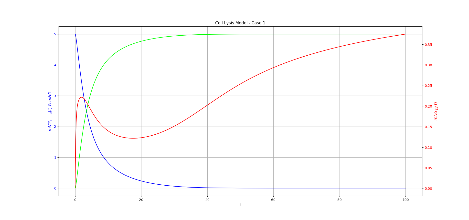
Figure 1: Case 1 of the cell lysis model. \(mNG_{1-10}\) is shown in blue, \(mNG_{11}\) is shown in red, and \(mNG\) is shown in lime. The chosen constants were: \(\theta = 1.0\), \(\mu=0.0\), \(\beta=1.0\), \(\epsilon=2.0\), \(x=3.5\), and \(\tau=0.5\). Initial conditions \([mNG_{11}](0)= 0.0\) and \([mNG_{1-10}](0)=5.0\) were chosen for this. The functions were approximated using Runge-kutta methods and the figure made using Matplotlib.

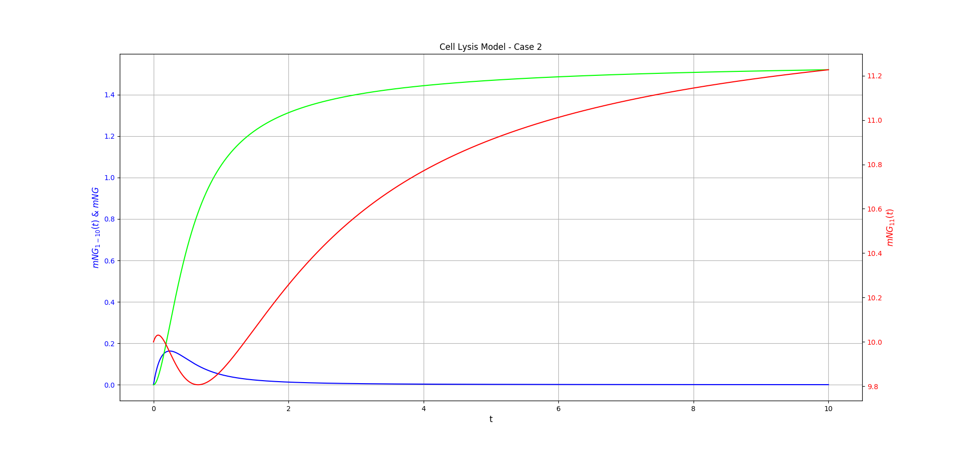
Figure 2: Case 2 of the cell lysis model. \(mNG_{1-10}\) is shown in blue, \(mNG_{11}\) is shown in red, and \(mNG\) is shown in lime. The chosen constants were: \(\theta = 1.0\), \(\mu=0.0\), \(\beta=1.0\), \(\epsilon=2.0\), \(x=2.0\), and \(\tau=0.5\). Initial conditions \([mNG_{11}](0)= 10.0\) and \([mNG_{1-10}](0)=0.0\) were chosen for this. The functions were approximated using Runge-kutta methods and the figure made using Matplotlib.

Biofilm model

The biofilm system uses binding proteins attached to fluorescent proteins to indicate prescence of biofilm by binding to specific target molecules. Hence, it suffices to consider only the action of the binding protein on the target molecule of choice, in this case denoted \(SpA\). \(PSL\) denotes the complementary target molecule for \(SpA\), but \(PSL\) could be substituted for Alginate or Cellulose, and \(SpA\) for their respective binding protein.

This model describes the rate at which \(SpA\) binds to the \(PSL\) polysaccharide, found in the biofilm. \( \phi\) represents the rate at which \(SpA\) enters the system (assumed constant), \(\psi\) represents the rate constant for \(SpA + PSL \rightarrow SpA.PSL\) ( \(SpA\) binding), and \(\tau\) represents the \(SpA\) that detaches from \(PSL\) and returns to the system.

\begin{align} \frac{d[SpA]}{dt} = \phi - \psi\frac{[PSL]}{[SpA.PSL]} + \tau[SpA.PSL]\\ \frac{d[SpA.PSL]}{dt} = \psi\frac{[PSL]}{[SpA.PSL]} - \tau[SpA.PSL] \end{align}

No constants were determined for this system.

Credits

Thank you very much to Dr Chris Hooley for his guidance, which was invaluable.

References

Schlosshauer, M. and Baker, D. (2004) ‘Realistic protein-protein association rates from a simple diffusional model neglecting long-range interactions, free energy barriers, and landscape ruggedness.’, Protein science : a publication of the Protein Society. Wiley-Blackwell, 13(6), pp. 1660–9. doi: 10.1110/ps.03517304.

Shaner, N. C. et al. (2013) ‘A bright monomeric green fluorescent protein derived from Branchiostoma lanceolatum’, Nature Methods, 10(5), pp. 407–409. doi: 10.1038/nmeth.2413.