We created a Python program that can be used to help researchers easily model reaction rates involving any two-step sequential enzymatic reactions, where a different enzyme catalyzes each step. Our software assumes both enzymes obey Michaelis-Menten kinetics. Researchers only have to input initial enzyme and substrate concentrations and the enzymatic activity in order to create an easy-to-visualize plot of substrate concentrations vs. time. Researchers can follow the documented directions on our wiki to change or add variables specific to their enzymatic reactions, in order to get the graphs of substrate concentrations over time they wish to model. We licensed our program with the OSI approved MIT License.
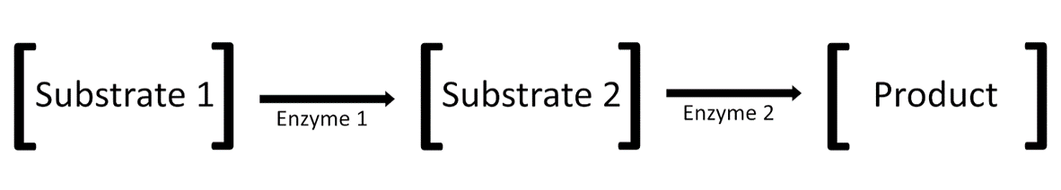
Figure 1-1. A schematic diagram of a general two-step sequential enzymatic reaction.
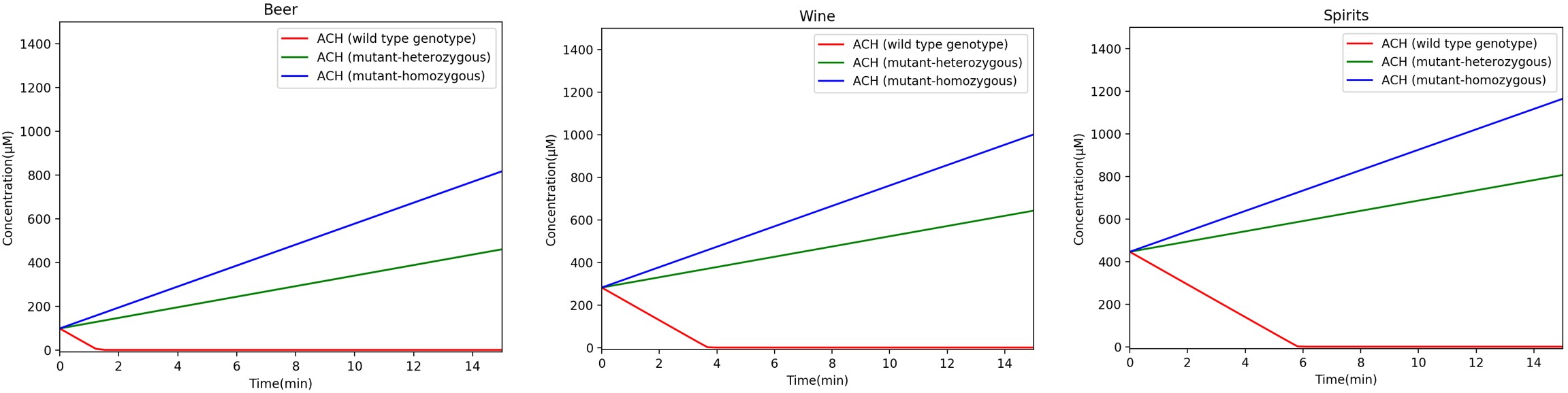
To show an example of how this software can be used, we modeled acetaldehyde concentrations in the mouth over time, for three different ALDH2 genotypes after consuming different alcoholic beverages.
We constructed a system of two differential equations to model the change in concentrations of ethanol and acetaldehyde in a human’s mouth over time based on the pathway illustrated in Figure 1-1.
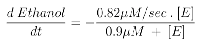
Equation 1 (above) models the change in ethanol concentration over time. We set it as equal to the enzymatic activity of ADH1B*2 enzymes. The symbol [E] represents ethanol concentration. This differential equation corresponds to the conversion rate of substrate 1 to substrate 2 in Figure 1-1.
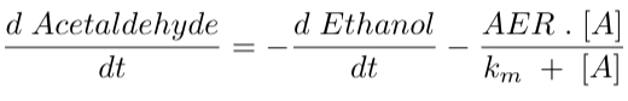
Equation 2 (above) models the change in acetaldehyde concentration over time. We set it as equal to the conversion rate of ethanol to acetaldehyde (d Ethanol/dt) minus the enzymatic activity of ALDH2 enzymes. The acetaldehyde elimination rate (AER) and km are constant values that vary for different ALDH2 genotypes. For example, a person who is homozygous wild type (ALDH2*1/*1) has an AER of 2.1 µM/sec and a Km of 0.2 µM (Rashkovetsky et al, 1994). The symbol [A] represents acetaldehyde concentration. This differential equation corresponds to the conversion rate of Substrate 2 to the Product in Figure 1-1.
There are three different ALDH2 genotypes (homozygous wild type ALDH2*1/*1; heterozygous ALDH2*1/*2; homozygous mutant ALDH2*2/*2), which process acetaldehyde at different rates (different Vmax values). Based on literature, we know that the heterozygous functions at 20-40% efficiency compared to homozygous wild type, while the homozygous mutant functions at 1-4% efficiency. The graphs below reflect the different efficiencies (20% and 1% were used to assume the worst case scenarios for the two mutant genotypes) (Gross et al., 2014; Chen et al., 2014).
Figure 1-2. Acetaldehyde concentration over time for three different types of alcohol (beer, wine, or spirits). The three curves in each graph represent acetaldehyde concentration over time for the different ALDH2 genotypes. Labels for each curve are provided in the legend.
As seen in Figure 1-2, in all three different alcoholic drinks, homozygous wild-type ALDH2*1/*1 metabolizes acetaldehyde the fastest, while the homozygous mutant ALDH2*2/*2 metabolizes acetaldehyde the slowest.
We hope that other researchers and teams will find this software tool useful for graphical visualizations of two-step sequential enzymatic reactions, where a different enzyme catalyzes each step.
Copy the source code (below) into a Python scriptfor use with Python 3.
Change variable values starting at line 34 to match those for your enzymes and substrates
Be especially careful that to check your units - all concentrations should be micromolar, and all times are in seconds.
Run and enjoy :)
Appendix: Source Code
#!/usr/bin/env python3
# -*- coding: utf-8 -*-
# -*- coding: utf-8 -*-
"""
Copyright <2018>
Permission is hereby granted, free of charge, to any person obtaining a copy of this software and associated documentation files (the "Two-step Enzymatic Reaction Solver"), to deal in the Software without restriction, including without limitation the rights to use, copy, modify, merge, publish, distribute, sublicense, and/or sell copies of the Software, and to permit persons to whom the Software is furnished to do so, subject to the following conditions:

The above copyright notice and this permission notice shall be included in all copies or substantial portions of the Software.

THE SOFTWARE IS PROVIDED "AS IS", WITHOUT WARRANTY OF ANY KIND, EXPRESS OR IMPLIED, INCLUDING BUT NOT LIMITED TO THE WARRANTIES OF MERCHANTABILITY, FITNESS FOR A PARTICULAR PURPOSE AND NONINFRINGEMENT. IN NO EVENT SHALL THE AUTHORS OR COPYRIGHT HOLDERS BE LIABLE FOR ANY CLAIM, DAMAGES OR OTHER LIABILITY, WHETHER IN AN ACTION OF CONTRACT, TORT OR OTHERWISE, ARISING FROM, OUT OF OR IN CONNECTION WITH THE SOFTWARE OR THE USE OR OTHER DEALINGS IN THE SOFTWARE.

@author: Justin Lin
"""
import numpy as np
import matplotlib.pyplot as plt

#Imports the Animation class for animated plots from matplot.lib
from matplotlib import animation
from scipy.integrate import solve_ivp

#### REAL TIME ANIMATION CODE AT THE BOTTOM :) ####

#### BEGIN EDITING HERE!!! ####

#Assigning axis and title names. Can change the texts (or units) within the string if needed
x_Axis = "Time(s)"
y_Axis = "Concentration(µM)"
title = "Concentration vs Time"

# Defining names, constants, and enzymatic activity for enzymes in µM/sec
v_max_enzyme_1 = 0.82
v_max_enzyme_2 = 2.1
km_enzyme_1 = 0.9
km_enzyme_2 = 0.2

# Defining initial substrates' concentrations.
# Add more variables if there are more steps and substrates in the reaction.
substrate_1_conc = 20 #in µM
substrate_2_conc = 15
substrate_1_name = "Ethanol"
substrate_2_name = "Acetaldehyde" #Enter names of substrates for plot's legends

# defining graph limits
low_y = 0 # in µM
high_y = 20

total_time = 20 # time of simulation in seconds. CAREFUL, if this is very long things will be slow

#REMEMBER, UNITS MUST BE CONSISTENT


##### DO NOT EDIT PAST THIS POINT UNLESS YOU KNOW WHAT YOU'RE DOING #####

#### Troubleshooting
# Increase the number of steps if your differential equation is not behaving
num_steps = total_time*5

# defining a function that returns the differential equations
def dX_dt(t, X):
    # Creating a tuple of the variables. Can add if there are more steps.
    E, A1= X
    # Setting up the differential equations
    v_enzyme_1 = -(v_max_enzyme_1*E)/(km_enzyme_1 + E)
    v_enzyme_2 = -(v_max_enzyme_2*A1)/(km_enzyme_2+A1)
    # The function returns a numpy array that stores the differential equations
    return np.array([(v_enzyme_1), (-v_enzyme_1+v_enzyme_2)])


# Returns an array of values (between 0 to final) that are evenly spaced according to the desired number of time steps
t = np.linspace(0, total_time, num_steps)

# Solves the differential equations. More substrate concentration values can simply be added to the list below if applicable.
# Integration method can be altered depending on the type of differential equations and the user.
result = solve_ivp(dX_dt, (t.min(), t.max()), [substrate_1_conc, substrate_2_conc], t_eval = t, method = "LSODA")


# Creating a "Figure" for the Cartesian plot
fig = plt.figure()
# Adjust plot domain and range size here
ax = fig.add_subplot(111, xlim=(0,total_time), ylim=(low_y, high_y))

# Add elements to plot here such as axis-title and graph title
ax.set_xlabel(x_Axis)
ax.set_ylabel(y_Axis)
ax.set_title(title)


# Plots the solution to our systemn of differential equations. Colors of the line can be customized.
# If there are more equations,
ax.plot(result.t, result.y[0], 'r-', label = substrate_1_name)
ax.plot(result.t, result.y[1], 'g-', label = substrate_2_name)

# Adds legend to the title
ax.legend()


##### This part can be uncommented if user wants a real time animated plot
'''
trace_x = []
trace_y1 = []
trace_y2 = []

# Creating a list of points that we're gonna plot
trace1 = ax.plot([],[],'b-', label = substrate_1_name)[0]
trace2 = ax.plot([],[], 'r-', label = substrate_2_name)[0]

# Defining a function that returns the argument
# --> basically what it does when the program moves on to plot the next point
def init():
    trace_x = []
    trace_y1 = []
    trace_y2 = []
    trace1.set_data(trace_x, trace_y1)
    trace2.set_data(trace_x, trace_y2)
    ax.legend(loc='upper right')
    #the commas after the lists are important because the commas make the list iterable
    #the commas are needed to allow the lists be read
    return trace1, trace2,

# Defining a function that returns the lists with the values appended (or added)
def animate(i):
    trace_x.append(result.t[i])
    trace_y1.append(result.y[0][i])
    trace1.set_data(trace_x, trace_y1)
    trace_y2.append(result.y[1][i])
    trace2.set_data(trace_x, trace_y2)
    return trace1, trace2,

#plots out the animated version
anim = animation.FuncAnimation(fig, animate, init_func=init, interval=50, blit=True)'''