Team:BostonU HW/Model
Modeling
Models are vital components to any engineering project because they simplify complex systems through a set of specified parameters. Mathematical models are especially useful because they can be used to predict a system’s behavior given certain inputs. For TERRA we have used several models to simulate the droplet formation at the end of an output tube and characterize our XY-translational plane.
 After comparing the experimental droplet volume to the theoretical droplet volume value at flow rates of 1 mL/hr, 2.5 mL/hr, 5 mL/hr, 7.5 mL/hr we learned two things:
 Zhang et al.
 In order to determine the correction factor we ran a series of experiments to calculate experimental droplet sizes at 15 different flow rates, following the data collection method outlined earlier. The flow rates tested are 0.5, 1, 1.5, 2, 2.5, 3, 3.5, 4, 4.5, 5, 6, 7, 8, 9, 10 mL/hr. For statistical significance we measured 30 droplet volumes per flow rate by measuring the time interval between droplets, using the same method for droplet volume calculation mentioned above. Finally, the correction factor, C, was isolated in the dynamic model and was calculated using the experimentally calculated droplet volume and other parameters from the dynamic model. These calculations were performed in a MATLAB script. The average correction factor for the 30 droplets for each flow rate was then calculated to obtain a final set of 15 empirically C values to see how they differed between flow rates. The plots below display the results of our modeling experiments
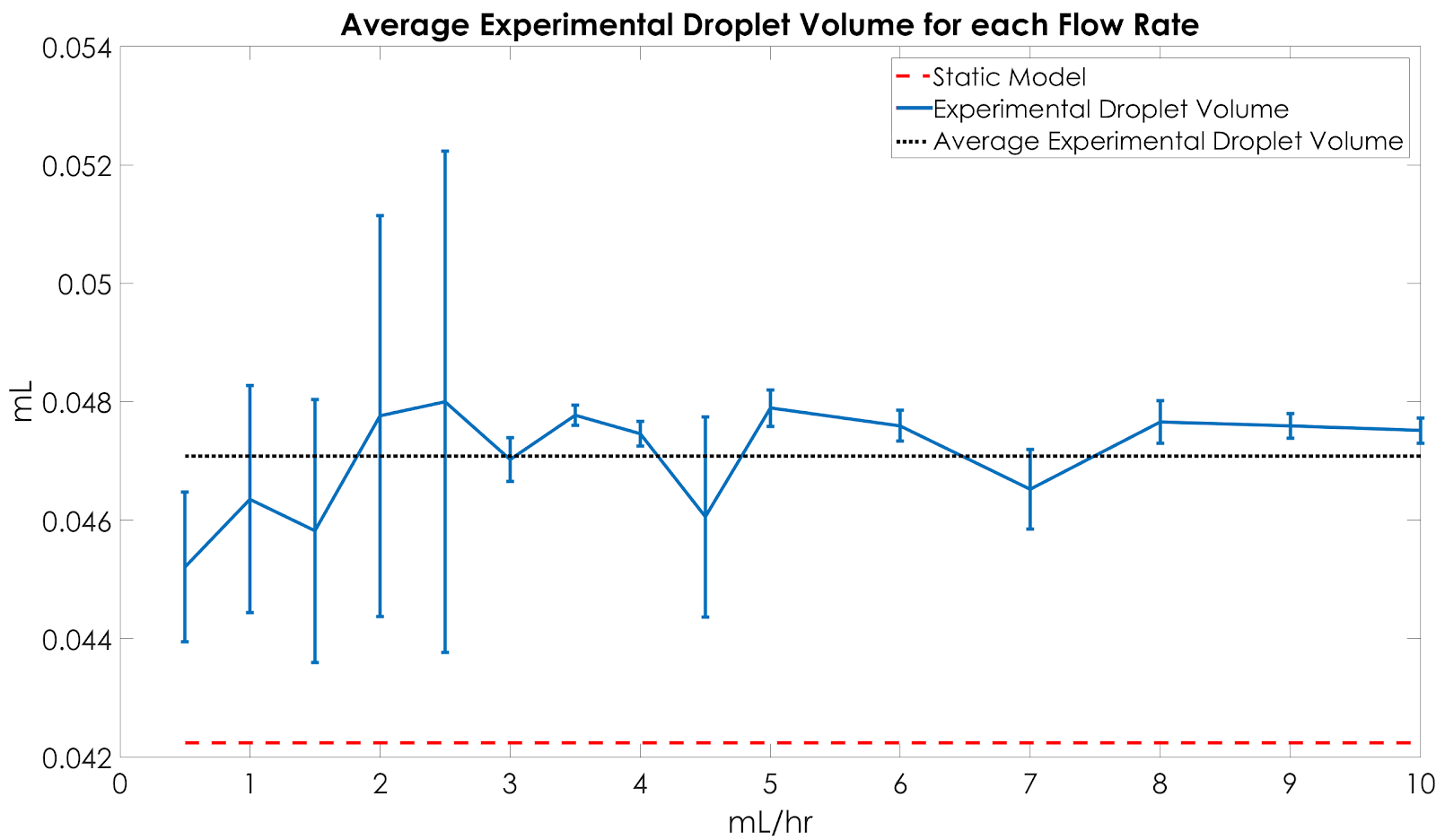 Figure 1. Plot of the average experimental droplet volume versus the predicted volume from the static model.
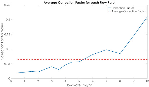 Figure 2. Plot of the correction factors calculate based on the experimental volumes at various flow rates against the average correction factor.
Unfortunately, these experiments did not result in a consistent correction factor that can be used across different flow rates. Instead, the correction factor on average increases across flow rates. While we observed an increase in droplet size as flow rate increased, we concluded that our current model lacks parameters that account for other physical phenomena in droplet formation and that more data was necessary to identify an empirical correction factor. However, we learned other important information to adjust the current static model. Because of this we decided to multiply the static model by a factor of 1.33 to account for the difference between average and static model.
References:
1 Zhang, D. F., and H. A. Stone. “Drop Formation in Viscous Flows at a Vertical Capillary Tube.” Physics of Fluids 9, no. 8 (August 1997): 2234–42. https://doi.org/10.1063/1.869346.
Figure 2. Plot of the correction factors calculate based on the experimental volumes at various flow rates against the average correction factor.
Unfortunately, these experiments did not result in a consistent correction factor that can be used across different flow rates. Instead, the correction factor on average increases across flow rates. While we observed an increase in droplet size as flow rate increased, we concluded that our current model lacks parameters that account for other physical phenomena in droplet formation and that more data was necessary to identify an empirical correction factor. However, we learned other important information to adjust the current static model. Because of this we decided to multiply the static model by a factor of 1.33 to account for the difference between average and static model.
References:
1 Zhang, D. F., and H. A. Stone. “Drop Formation in Viscous Flows at a Vertical Capillary Tube.” Physics of Fluids 9, no. 8 (August 1997): 2234–42. https://doi.org/10.1063/1.869346.
Next, we measured the circumference of our pulley.
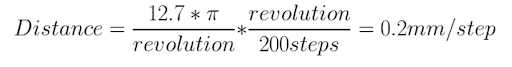
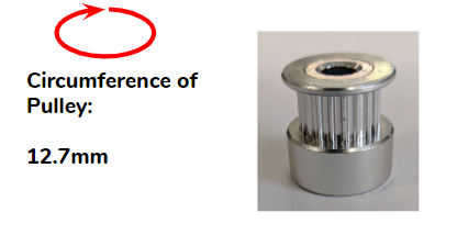 After obtaining these values, we found the distance it is possible to travel per step, and finally the steps per well. From the documentation for the NEMA-14 stepper motor, we know it steps 200 times in one revolution and has microstepping features up to 1/32 microsteps.
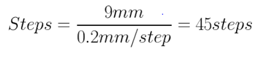 From there, since we know how many steps is required for 96 wells, we calculate the microtiter plates with different amounts of wells.

Terra averages around 8 runs before it requires a reset. A reset consists of rehoming the device from its starting point, readjusting the tubing, and resetting the plate on the plane.
The average time taken to transverse the 108 mm was 39.306 seconds. From that, we determined that, with a microstep of 1/4 steps, the XY-stage moves at an average speed of 2.75 mm/sec. The average time taken to travel between wells on a 96 well plate was 3.28 seconds. Since the time taken to travel is dependent on the distance between the center of each well, we can extrapolate from this data to find the average time taken to travel from well-to-well on multiple types of microtiter plates.
Droplet Characterization
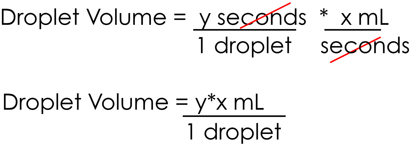
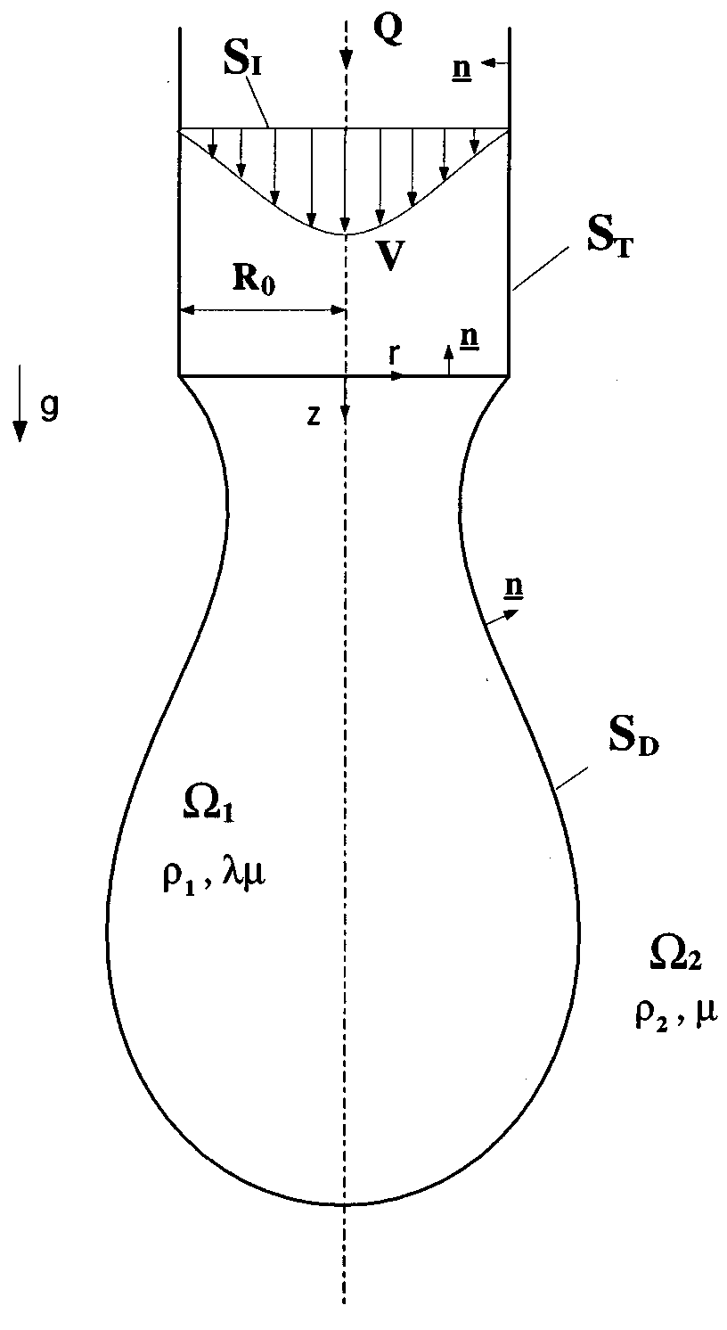
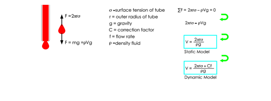
Due to the relatively low flow rate that fluid moves at in microfluidic chips, outputs dispensed from microfluidic chips are typically droplets rather than a continuous stream. Therefore, in order to accurately dispense these droplets into wells, we created a model to predict their volume so that users can have greater control of the end sample volume in the well of interest. To develop the model we used a free-body diagram to identify the forces present right before a droplet falls off the nozzle. Using the sum of the forces acting on the droplet we were able to model the its theoretical volume. The derivation of the static model is shown below. To test the model we ran preliminary experiments to calculate volumes at flow rates of 1 mL/hr, 2.5 mL/hr, 5 mL/hr, 7.5 mL/hr and compared them against the theoretical value. To calculate droplet volumes we followed the following method:- Set up a single syringe pump with a 12 mL syringe filled with red colored water. The tubing is then passed through the nozzle of TERRA to stabilize the tubing. A well plate is then placed under the tubing to catch droplets.
- Start the syringe pump at the flow rate of interest.
- Place a smartphone on a flat surface that captures the droplet falling off the tubing and hitting the well plate.
- Start recording the droplets dispensing, ensuring that it left at a duration long enough to capture at least 35 droplets.
- Analyze the video by measuring the time interval between droplets.
- The theoretical volume from the model was less than the experimental.
- This difference, on average, increased with flow rate.
A potential reason for the missing parameters is that the model assumed that the fluid is static instead of dynamic, due to the constant flow rate of fluid moving through the chip.1 In a dynamic model, the total droplet volume is characterized by the static volume and the pinching volume.1 The pinching volume is formed during the droplet’s fall when the droplet breaks off the tube.1
However, after researching the physical phenomenon behind dynamic droplets we realized that a complete dynamic model, as described in Zhang et al, requires complicated parameters, such as the fluid interface, making it difficult to implement.1 Therefore, we decided to create our dynamic model empirically by adding a correction factor, which would depend mainly on flow rate.
Zhang et al.
In order to determine the correction factor we ran a series of experiments to calculate experimental droplet sizes at 15 different flow rates, following the data collection method outlined earlier. The flow rates tested are 0.5, 1, 1.5, 2, 2.5, 3, 3.5, 4, 4.5, 5, 6, 7, 8, 9, 10 mL/hr. For statistical significance we measured 30 droplet volumes per flow rate by measuring the time interval between droplets, using the same method for droplet volume calculation mentioned above. Finally, the correction factor, C, was isolated in the dynamic model and was calculated using the experimentally calculated droplet volume and other parameters from the dynamic model. These calculations were performed in a MATLAB script. The average correction factor for the 30 droplets for each flow rate was then calculated to obtain a final set of 15 empirically C values to see how they differed between flow rates. The plots below display the results of our modeling experiments
Distance Traveled to Dispense Fluid
In order to accurately dispense the output into the desired wells, the plane needed to travel the right amount of steps depending on the well plate. Therefore we needed to calculate how many steps of the stepper motor is required to move from one well to another. Below are the steps and calculations that went into determining this: To do so, we first determined the distance from center of well to next center well for each microtiter plate.Next, we measured the circumference of our pulley.
| Well Plate | Dimensions | Steps/Well |
|---|---|---|
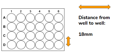
| 24-well plate | 4x6 wells (18 mm apart) | 90 steps |
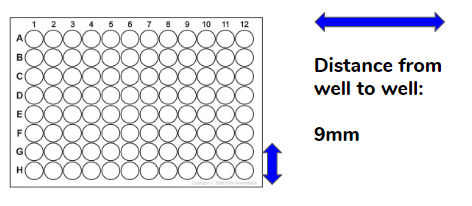
| 96-well plate | 8x12 wells (9 mm apart) | 45 steps |
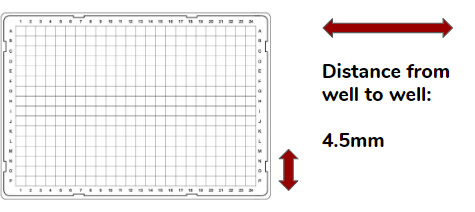
| 384-well plate | 16x24 wells (4.5 mm apart) | 22.5 steps |
Runs Before Failure
To characterize the amount of runs the XY-stage can perform before failure, we ran TERRA through a set of 15 trials in which fluid was dispensed into two different wells ten times. These trials were run independently from each other by resetting TERRA in between trials. In each trial, two outputs were simulated--one outputting at location 45, and the latter outputting at location 90. The experiments allowed us to understand how many loops TERRA would run through before it fails to output into a correct well location, and therefore requires a reset.
Terra averages around 8 runs before it requires a reset. A reset consists of rehoming the device from its starting point, readjusting the tubing, and resetting the plate on the plane.
Speed and Time
A set of 15 trials were run in order to determine the speed of the plate support of the XY-stage. The plate support traveled a distance of 108mm. The time taken to travel was recorded for each trial and then averaged. To calculate the average speed, the distance traveled was divided by the time per run.
The average time taken to transverse the 108 mm was 39.306 seconds. From that, we determined that, with a microstep of 1/4 steps, the XY-stage moves at an average speed of 2.75 mm/sec. The average time taken to travel between wells on a 96 well plate was 3.28 seconds. Since the time taken to travel is dependent on the distance between the center of each well, we can extrapolate from this data to find the average time taken to travel from well-to-well on multiple types of microtiter plates.
| Well Plate | Distance from Center of Wells | Time Required |
|---|---|---|
| 24-well plate | 18 mm apart | 6.56 seconds |
| 96-well plate | 9 mm apart | 3.28 seconds |
| 384-well plate | 4.5 mm apart | 1.64 seconds |