Overview
We will introduce how we use knowledge of mathematics and algorithms to implement function of Alpha Ant in details in this section. It consists of three parts, Pathway Search Algorithm, Pathway Ranking Methods and Additional functions.Search Algorithm: DFSSeeking for biosynthesis pathways from the starting material to the product is a typical search problem. We abstracted the original biosynthesis pathway search problem and turned it into a directed graph search problem.First we built a directed graph that models the transformation of metabolites where its vertices represent metabolites and its edges represent chemical transformations via reactions. Fig.1. Search algorithm:DFS(Depth-first Search)Then we used the Depth-first search algorithm to traverse and search this graph data structures. Not only do we need to get all of the solutions that satisfy the constraints, but also need to record the search path. The DFS algorithm starts at the root node and explores as far as possible along each branch before backtracking. The search remembers previously visited nodes and will not repeat them therefore avoiding infinite loop. As a result, all solutions that satisfy the constraints will be returned. The procedure of DFS is described as follows:Fig.2. The procedure of DFSThe reason we choose this algorithm is that it can solve the pathway search problem efficiently. Based on adjacency matrix, DFS algorithm can solve the problem within the time complexity of O (E + V).[1] ‘E’ means the number of edges and ‘V’ means the number of vertex, and we are able to solve the problem by traversing all the edges and vertex just only once. Moreover, the core algorithm of DFS is flexible, so that we can combine it with other evaluation algorithms to solve more complex problems.Pathway Ranking CriteriaWe adopt three criteria to evaluate the efficacy of the pathways which are thermodynamic feasibility& precursor competition, toxicity of metabolites and atom conservation. After grading pathway using different criteria, we normalize the scores and give users the right to define different weights of different ranking criteria.The criterion of thermodynamic feasibility& precursor competition:We use a statistical mechanical model to present the competition for a metabolic precursor with endogenous reactions. We compute the probability of each reaction with ∆_r G^('°) ( the standard reaction Gibbs free energy) through the Boltzmann distribution according to study of Hiroyuki Kuwahara et.al[2]. Here is the mathematical description.Fig.3. We consider C as the metabolic precursor. Let RN be a set of native reactions that can transform C in a given host organism and Rr is the reaction in the pathway to be evaluated.The Boltzmann factor of reaction r that can transform C :\[{{\rm{e}}^{ - {\Delta _r}{G^{' \circ /RT}}}}\](Equation 1.1)We define the normalized Boltzmann factor for r as f(r) :∆_r G^('°): the standard reaction Gibbs energy
RN: a set of native reactions that can transform C in a given host organism
R : gas constant
T : absolute temperature(Equation 1.2)If r∈R_N , then f(r) is simply based on the Boltzmann distribution of the native reaction system transforming compound C. If r∉R_N, then f(r) is based on the Boltzmann distribution of the reaction system that contains all native reactions transforming C and foreign reaction r.Fig.4. Gibbs standard energy data distribution.For each pathway, every reaction r in the pathway has the score log f(r),The score of the pathway is as follows:\[S = \log f(r1) + \log f(r2) + ... + \log f(rn)\](Equation 1.3)Every reaction r in the pathway has the score log f(r),S refers to total score.S is used to evaluate the pathway. The higher the score is, the better the pathway is.\[{S_{total}} = \left( {\begin{array}{*{20}{c}}{{S_{\;th}}}&{{S_t}}&{{S_f}}\end{array}} \right)\left( {\begin{array}{*{20}{c}}{{w_{th}}}\\{{w_t}}\\{{w_f}}\end{array}} \right)\](Equation 1.4)The equation above show how the total score is calculated. Corresponding to each ranking criteria, we give them a certain weight.Of course, users can adjust the weight as well. Consequently, the result list is arranged in descending order of total score.Standardization of scoreGraphs below show the distribution of our data.In order to elimate the influence of exceptional data, we use pauta criterion to calculate the upper and lower limit according to average value and variance.\[\begin{array}{l}\mu {\rm{ = }}\frac{1}{n}\sum\limits_{i = 1}^n {arra{y_i}} \\\sigma = \frac{1}{n}\sum\limits_{i = 1}^n {{{(arra{y_i} - \mu )}^2}} \\lower = \mu - 3\sigma \\upper = \mu + 3\sigma \end{array}\](Equation 1.5)\[\begin{array}{l}arra{y_i} = \left\{ \begin{array}{l}lower,{\rm{ }}arra{y_i} < lower\\arra{y_i},{\rm{ }}lower \le arra{y_i} \le upper\\upper,{\rm{ }}arra{y_i} > upper\end{array} \right.\\{\rm{array = }}\left( {array - \mu } \right)/\sigma \end{array}\](Equation 1.6)The distribution of reaction frequency is skewed, cause most reactions can only endogenously construct in a few organisms, which leads to the unbalance of score values. So before turning the frequency data into the standard normal distribution, we use ln(x) to process it to get a more reliable result.We adjust the score array by the limits and turn it into the standard normal distribution. So that all the scores of different criteria are on the same scale, and we can calculate the total score through weighted summation method.Additional function algorithmMicroorganism recommendationAfter searching the pathways, we first select n(n is defined by users) pathways ranking by sum of free Gibbs energy and then use previous scoring method to calculate each route’s score of certain organism. Next we rank the average score of all species and the highest is the best. The number of the selected pathways n can be defined by users. The default value is 50.Fig.5. At first, search all possible pathway by using DFS.then use previous scoring method to calculate each route’s score of certain organism. Next we rank the average score of all species and the highest is the best. The number of the selected pathways n can be defined by users.The average score of every organism:\[Ave(A) = \frac{{\sum\limits_{i = 1}^n {Score{A_i}} }}{n}\](Equation 2.1)The organism with highest score will be the best.\[{Max\left\{ {Ave(A),Ave(B),Ave(C),Ave(D)...} \right\}\begin{array}{*{20}{c}}{}&{}\end{array}}\](Equation 2.2)Flux balance analysis(FBA)Flux balance analysis is a mathematical approach for analyzing the flow of metabolites through a metabolic network. It required very little information in terms of the enzyme kinetic parameters and concentration of metabolites in the system in contrast to the traditionally followed approach of metabolic modeling using coupled ordinary differential equations.[3] FBA achieves this by making two assumptions, steady state and optimality.Assumption 1: The modeled system has entered a steady state, where the metabolite concentrations no longer change, i.e. in each metabolite node the producing and consuming fluxes cancel each other out.Assumption 2: The organism has been optimized through evolution for some biological goal, such as optimal growth or conservation of resources.We use the COBRApy package to implement the function of FBA. [4]The following are illustrations of flux balance analysis.First we construct a new model based on a model of E. coli core metabolism. This genome-scale metabolic network contains the core metabolism reactions in E. coli. When we need to construct novel reactions into E.coli, we can add the reactions in Systems Biology Markup Language(SBML) which is an XML-based standard format for distributing models supporting for COBRA models through the FBC extension version 2.Fig.6. First we construct a new model based on a model of E. coli core metabolism. This genome-scale metabolic network contains the core metabolism reactions in E. coli. Then we present metabolic reactions as a stoichiometric matrix (S) of size m × n. Every row of this matrix represents one unique compound (for a system with m compounds) and every column represents one reaction (n reactions). The entries in each column are the stoichiometric coefficients of the metabolites participating in a reaction. There is a negative coefficient for every metabolite consumed and a positive coefficient for every metabolite that is produced. A stoichiometric coefficient of zero is used for every metabolite that does not participate in a particular reaction.Fig.7.we present metabolic reactions as a stoichiometric matrix (S) of size m × n. Every row of this matrix represents one unique compound (for a system with m compounds) and every column represents one reaction (n reactions). Constraints are represented in two ways, as equations that present steady-state mass balance and as inequalities that impose bounds on the system.The concentrations of all metabolites are represented by the vector x, with length m. The flux through all of the reactions in a network is represented by the vector v, which has a length of n. A steady-state mass balance constraint was imposed according to assumption 1.\[\begin{array}{l}dX/dt = 0\\
{\rm{ }}S \times v = 0\end{array}\](Equation 3.1)Every reaction will be given upper and lower bounds, which define the maximum and minimum allowable fluxes of the reactions. In our software, v_^Upper was set to 1000 mmol/gDW/hour and v_^Lower was set to 0 or -1000 mmol/gDW/hour for irreversible and reversible reactions, respectively.\[{\rm{ }}{v^{Lower}} \le {v_i} \le {v^{Upper}}\](Equation 3.2)The next step is to define the objective function. It can be any linear combination of fluxes, where c is a vector of weights indicating how much each reaction (such as the biomass reaction when simulating maximum growth) contributes to the objective function. This function is defined by users.\[Z = {c^T}v\](Equation 3.3)Last we use linear programming to identify a flux distribution that maximizes or minimizes the objective function within the space of allowable fluxes defined by the constraints imposed by the mass balance equations and reaction bounds.Similarity Comparison of CompoundWe use Extended-Connectivity Fingerprints (ECFPs) to present the structure of compound for molecular similarity searching. ECFPs represent molecular structures by means of circular atom neighborhoods.[5]Representation:The representation of ECFPs is by means of varying-length lists of integer identifiers. Each identifier represents a particular substructure, more precisely, a circular atom neighborhood, which is present in the molecule. This identifier captures some local information about the corresponding atom in such a way that various atom properties (e.g., atomic number, connection count, etc.) are packed into a single integer value using a hash function. [5]The list of integer identifiers is sorted in ascending order. Then the identifier list is converted to the fixed length bit string.[6]Fig.8. ECFP generation process.Fig.9. Generation of the fixed-length bit string ("folding")More information could be found in here.We turn the fixed-length binary of a compound into an array. We use dice coefficient to evaluate the similarity of two compounds, which is a function to measure the set similarity.Length: This parameter specifies the length of the bit string representation. The default length is 1024.a: Array of compound a
b: Array of compound b
\[{\rm{ }}Dice(a,b) = \frac{{2 \times \sum\limits_{i = 1}^{length(a)} {commo{n_i}(a,b)} }}{{length(a) + length(b)}}\](Equation 4.1)\[commo{n_i}(a,b) = \left\{ \begin{array}{l}1,{\rm{ }}\begin{array}{*{20}{c}}{}\end{array}{{\rm{a}}_i} = {b_i}\\0{\rm{, }}\begin{array}{*{20}{c}}{}\end{array}{{\rm{a}}_i} \ne {b_i}\end{array} \right.\](Equation 4.2)Atom conservationThere is a one-to-one correspondence between atom index from reactant and atom index from product in MetaCyc. We integrated the data form into the main pairs in KEGG. We cleaned and removed the redundant data. In one pathway, each step of the reaction is recursive, leaving only the atomic number derived from the source compound, and the rest of the positions are -1. Finally, you can calculate how many atoms in the target are from the source compound.In order to calculate the final atom conservation rate in a pathway, we need to figure out a data format to describe the atom transferring. In our data format, we create an array for each reactant and product. Every atom in the product has a specific position which is labeled as a sequential array. Each number in the array of reactant means the position of the target compound that atom will transfer to.Fig.10. Some concepts we define in a certain pathway.\[T(i,source,target) = \left\{ \begin{array}{l} - 1{\rm{ , }}\begin{array}{*{20}{c}}{}&{}\end{array}{\rm{ }}{{\rm{i}}^{th}}{\rm{ atom}}\begin{array}{*{20}{c}}{}\end{array}{\rm{of}}\begin{array}{*{20}{c}}{}\end{array}{\rm{source}}\begin{array}{*{20}{c}}{}\end{array}{\rm{doesn't}}\begin{array}{*{20}{c}}{}\end{array}{\rm{transfer}}\begin{array}{*{20}{c}}{}\end{array}{\rm{to}}\begin{array}{*{20}{c}}{}\end{array}{\rm{target}}\\x{\rm{ , }}\begin{array}{*{20}{c}}{}&{}\end{array}{\rm{ }}{{\rm{i}}^{th}}{\rm{ atom}}\begin{array}{*{20}{c}}{}\end{array}{\rm{of}}\begin{array}{*{20}{c}}{}\end{array}{\rm{source}}\begin{array}{*{20}{c}}{}\end{array}{\rm{transfers}}\begin{array}{*{20}{c}}{}\end{array}{\rm{to}}\begin{array}{*{20}{c}}{}\end{array}{\rm{the}}\begin{array}{*{20}{c}}{}\end{array}{{\rm{x}}^{th}}\begin{array}{*{20}{c}}{}\end{array}{\rm{atom}}\begin{array}{*{20}{c}}{}\end{array}{\rm{of}}\begin{array}{*{20}{c}}{}\end{array}{\rm{target}}\end{array} \right.\](Equation 5.1)\[\begin{array}{l}{{\rm{R}}_j}(i) = T(i,{{\rm{R}}_{\rm{j}}}{\rm{,}}{{\rm{P}}_{\rm{j}}}{\rm{) }}\begin{array}{*{20}{c}}{}&{}\end{array}{\rm{ i = 1,2, }}...{\rm{ , A(}}{{\rm{R}}_{\rm{j}}}{\rm{) }}\begin{array}{*{20}{c}}{}&{}\end{array}{\rm{ j = 1,2, }}...{\rm{ , n}}\\{\rm{ }}{{\rm{P}}_j}(i) = T(i,{{\rm{P}}_j}{\rm{,}}{{\rm{R}}_{\rm{j}}}{\rm{) }}\begin{array}{*{20}{c}}{}&{}\end{array}{\rm{ i = 1,2, }}...{\rm{ , A(}}{{\rm{P}}_{\rm{j}}}{\rm{) }}\begin{array}{*{20}{c}}{}&{}\end{array}{\rm{ j = 1,2, }}...{\rm{ , n}}\end{array}\](Equation 5.2)where Rj denotes the nth reactant, Rj(i) denotes the ith number of the Rj array, n denotes the amount of reactants in this pathway, A(Rj) denotes the amount of atoms in Rj. Other symbols with P have the same meanings about product.\[{{\rm{R}}_{{\rm{j + 1}}}}(i) = \left\{ \begin{array}{l} - 1,\begin{array}{*{20}{c}}{}&{}&{}&{}&{}&{}&{}&{}&{}\end{array}{{\rm{P}}_{\rm{j}}}(i) = - 1\\T(i,{\rm{reactant,product),}}\begin{array}{*{20}{c}}{}&{}\end{array}{{\rm{P}}_{\rm{j}}}(i) \ne - 1\end{array} \right.\](Equation 5.3)Since the jth product is the (j+1)th reactant in the same pathway, the Rj+1 array should be adjusted according to the Pn array. Only the atoms from nth reactant can transfer to the (j+1)th reactant. In this way we can find out how many atoms are conserved through our data format.\[\begin{array}{l}{\rm{C(}}{{\rm{R}}_{\rm{j}}}(i)) = \left\{ \begin{array}{l}0,{\rm{ }}{{\rm{R}}_{\rm{j}}}(i) = - 1\\1,{\rm{ }}{{\rm{R}}_{\rm{j}}}(i) \ne - 1{\rm{ }}\end{array} \right.\begin{array}{*{20}{c}}{}&{}\end{array}i = 1,2,...,{\rm{ A(}}{{\rm{R}}_{\rm{j}}}{\rm{)}}\\{\rm{ C(}}{{\rm{P}}_{\rm{j}}}(i)) = \left\{ \begin{array}{l}0,{\rm{ }}{{\rm{P}}_{\rm{j}}}(i) = - 1\\1,{\rm{ }}{{\rm{P}}_{\rm{j}}}(i) \ne - 1{\rm{ }}\end{array} \right.\begin{array}{*{20}{c}}{}&{}\end{array}i = 1,2,...,{\rm{ A(}}{{\rm{P}}_{\rm{j}}}{\rm{)}}\end{array}\](Equation 5.4)\[{\rm{ }}Atom\begin{array}{*{20}{c}}{}\end{array}conservation\begin{array}{*{20}{c}}{}\end{array}rate{\rm{ = }}\frac{{\sum\limits_{{\rm{i = 1}}}^{{\rm{A(}}{{\rm{P}}_{\rm{n}}}{\rm{)}}} {{\rm{C(}}{{\rm{P}}_{\rm{n}}}(i))} }}{{{\rm{A}}({R_1})}} \times 100\% \](Equation 5.5)At last, we can calculate the atom conservation rate through the first reactant array and the final product array.References:
[1] Rogers, D.; Hahn, M. Extended-Connectivity Fingerprints. J. Chem. Inf. Model. 2010, 50(5): 742-754.
[2] Hiroyuki Kuwahara, Meshari Alazmi, Xuefeng Cui and Xin Gao. MRE: a web tool to suggest foreign enzymes for the biosynthesis pathway design with competing endogenous reactions in mind. Nucleic Acids Research, 2016, Vol. 44, Web Server issue W217–W225.
[3] Orth, J.D.; Thiele, I.; Palsson, B.Ø. (2010). "What is flux balance analysis?". Nature Biotechnology. 28: 245–248. doi:10.1038/nbt.1614. PMC 3108565 Freely accessible. PMID 20212490
[4] Schellenberger J, Que R, Fleming RMT, Thiele I, Orth JD, Feist AM, Zielinski DC, Bordbar A, Lewis NE, Rahmanian S et al., Quantitative prediction of cellular metabolism with constraint-based models: the COBRA Toolbox v2.0 Nature Protocol, 2011,6(9):1290-307.
[5] Rogers, D.; Hahn, M. Extended-Connectivity Fingerprints. J. Chem. Inf. Model. 2010, 50(5): 742-754.
[6] Morgan, H. L. The Generation of a Unique Machine Description for Chemical Structures - A Technique Developed at Chemical Abstracts Service. J. Chem. Doc. 1965, 5: 107-112.


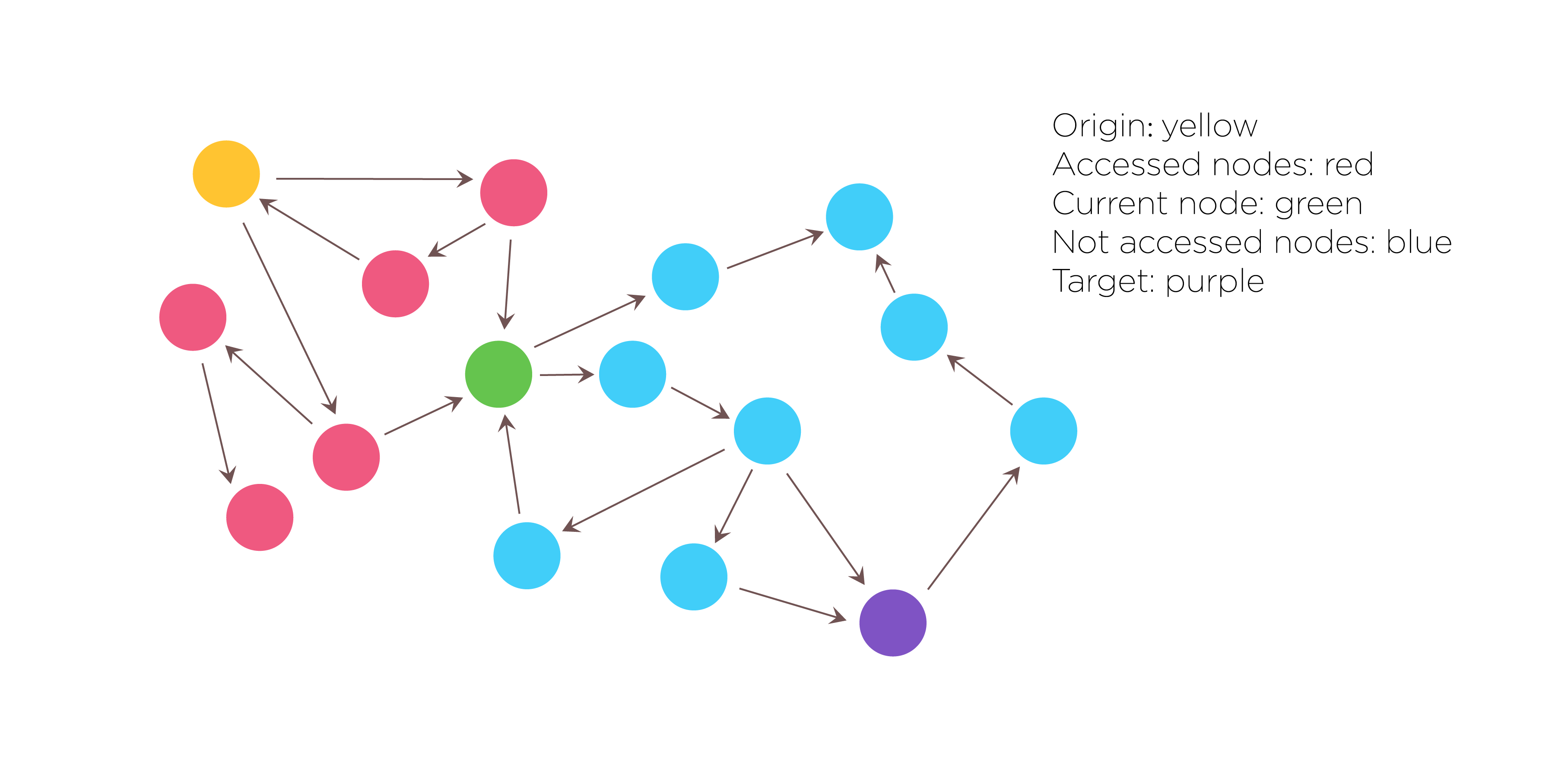 Fig.1. Search algorithm:DFS(Depth-first Search)
Then we used the Depth-first search algorithm to traverse and search this graph data structures. Not only do we need to get all of the solutions that satisfy the constraints, but also need to record the search path. The DFS algorithm starts at the root node and explores as far as possible along each branch before backtracking. The search remembers previously visited nodes and will not repeat them therefore avoiding infinite loop. As a result, all solutions that satisfy the constraints will be returned.
The procedure of DFS is described as follows:
Fig.1. Search algorithm:DFS(Depth-first Search)
Then we used the Depth-first search algorithm to traverse and search this graph data structures. Not only do we need to get all of the solutions that satisfy the constraints, but also need to record the search path. The DFS algorithm starts at the root node and explores as far as possible along each branch before backtracking. The search remembers previously visited nodes and will not repeat them therefore avoiding infinite loop. As a result, all solutions that satisfy the constraints will be returned.
The procedure of DFS is described as follows:
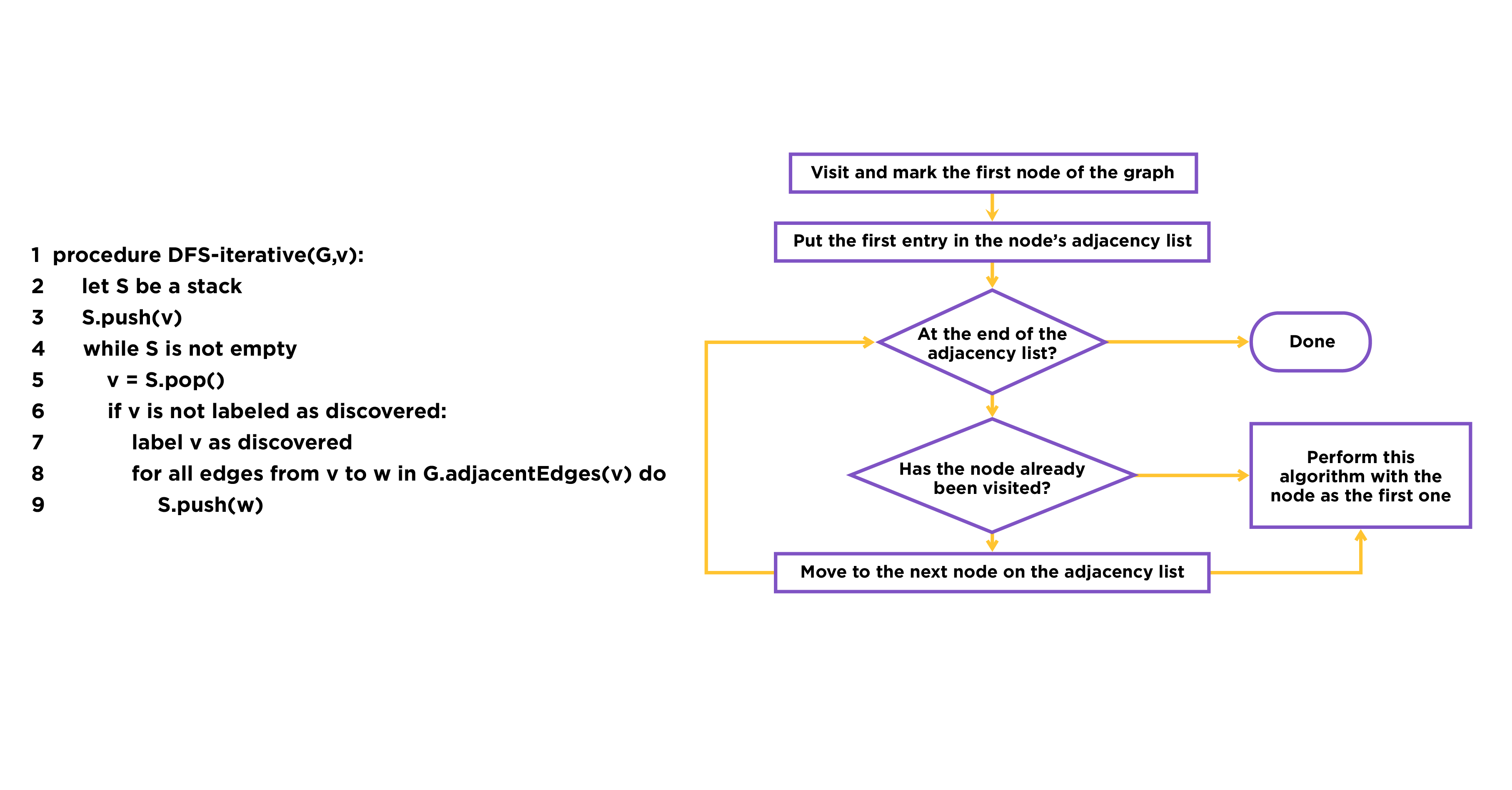 Fig.2. The procedure of DFS
The reason we choose this algorithm is that it can solve the pathway search problem efficiently. Based on adjacency matrix, DFS algorithm can solve the problem within the time complexity of O (E + V).[1] ‘E’ means the number of edges and ‘V’ means the number of vertex, and we are able to solve the problem by traversing all the edges and vertex just only once. Moreover, the core algorithm of DFS is flexible, so that we can combine it with other evaluation algorithms to solve more complex problems.
Pathway Ranking Criteria
We adopt three criteria to evaluate the efficacy of the pathways which are thermodynamic feasibility& precursor competition, toxicity of metabolites and atom conservation. After grading pathway using different criteria, we normalize the scores and give users the right to define different weights of different ranking criteria.
The criterion of thermodynamic feasibility& precursor competition:
We use a statistical mechanical model to present the competition for a metabolic precursor with endogenous reactions. We compute the probability of each reaction with ∆_r G^('°) ( the standard reaction Gibbs free energy) through the Boltzmann distribution according to study of Hiroyuki Kuwahara et.al[2]. Here is the mathematical description.
Fig.2. The procedure of DFS
The reason we choose this algorithm is that it can solve the pathway search problem efficiently. Based on adjacency matrix, DFS algorithm can solve the problem within the time complexity of O (E + V).[1] ‘E’ means the number of edges and ‘V’ means the number of vertex, and we are able to solve the problem by traversing all the edges and vertex just only once. Moreover, the core algorithm of DFS is flexible, so that we can combine it with other evaluation algorithms to solve more complex problems.
Pathway Ranking Criteria
We adopt three criteria to evaluate the efficacy of the pathways which are thermodynamic feasibility& precursor competition, toxicity of metabolites and atom conservation. After grading pathway using different criteria, we normalize the scores and give users the right to define different weights of different ranking criteria.
The criterion of thermodynamic feasibility& precursor competition:
We use a statistical mechanical model to present the competition for a metabolic precursor with endogenous reactions. We compute the probability of each reaction with ∆_r G^('°) ( the standard reaction Gibbs free energy) through the Boltzmann distribution according to study of Hiroyuki Kuwahara et.al[2]. Here is the mathematical description.
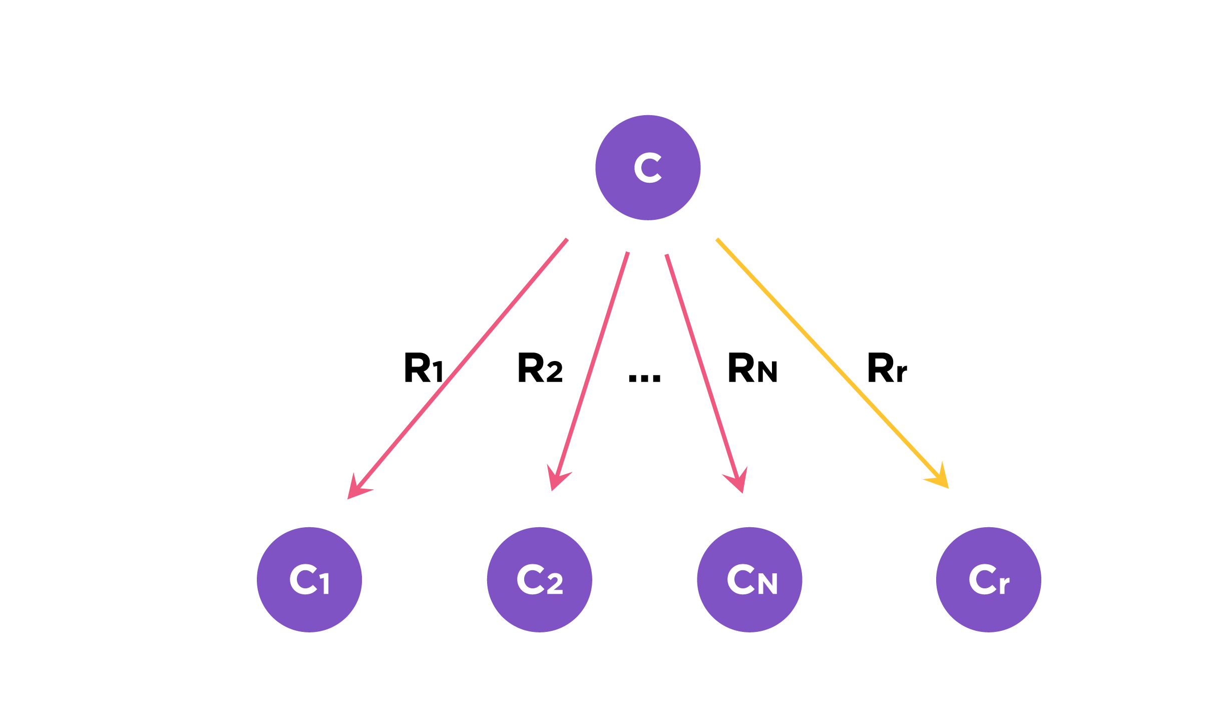 Fig.3. We consider C as the metabolic precursor. Let RN be a set of native reactions that can transform C in a given host organism and Rr is the reaction in the pathway to be evaluated.
The Boltzmann factor of reaction r that can transform C :
\[{{\rm{e}}^{ - {\Delta _r}{G^{' \circ /RT}}}}\]
(Equation 1.1)
We define the normalized Boltzmann factor for r as f(r) :
∆_r G^('°): the standard reaction Gibbs energy
RN: a set of native reactions that can transform C in a given host organism
R : gas constant
T : absolute temperature
Fig.3. We consider C as the metabolic precursor. Let RN be a set of native reactions that can transform C in a given host organism and Rr is the reaction in the pathway to be evaluated.
The Boltzmann factor of reaction r that can transform C :
\[{{\rm{e}}^{ - {\Delta _r}{G^{' \circ /RT}}}}\]
(Equation 1.1)
We define the normalized Boltzmann factor for r as f(r) :
∆_r G^('°): the standard reaction Gibbs energy
RN: a set of native reactions that can transform C in a given host organism
R : gas constant
T : absolute temperature
 (Equation 1.2)
If r∈R_N , then f(r) is simply based on the Boltzmann distribution of the native reaction system transforming compound C. If r∉R_N, then f(r) is based on the Boltzmann distribution of the reaction system that contains all native reactions transforming C and foreign reaction r.
(Equation 1.2)
If r∈R_N , then f(r) is simply based on the Boltzmann distribution of the native reaction system transforming compound C. If r∉R_N, then f(r) is based on the Boltzmann distribution of the reaction system that contains all native reactions transforming C and foreign reaction r.
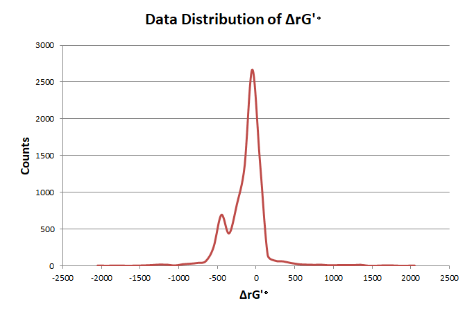
 Fig.4. Gibbs standard energy data distribution.
For each pathway, every reaction r in the pathway has the score log f(r),The score of the pathway is as follows:
\[S = \log f(r1) + \log f(r2) + ... + \log f(rn)\]
(Equation 1.3)
Every reaction r in the pathway has the score log f(r),S refers to total score.S is used to evaluate the pathway. The higher the score is, the better the pathway is.
\[{S_{total}} = \left( {\begin{array}{*{20}{c}}{{S_{\;th}}}&{{S_t}}&{{S_f}}\end{array}} \right)\left( {\begin{array}{*{20}{c}}{{w_{th}}}\\{{w_t}}\\{{w_f}}\end{array}} \right)\]
(Equation 1.4)
The equation above show how the total score is calculated. Corresponding to each ranking criteria, we give them a certain weight.Of course, users can adjust the weight as well. Consequently, the result list is arranged in descending order of total score.
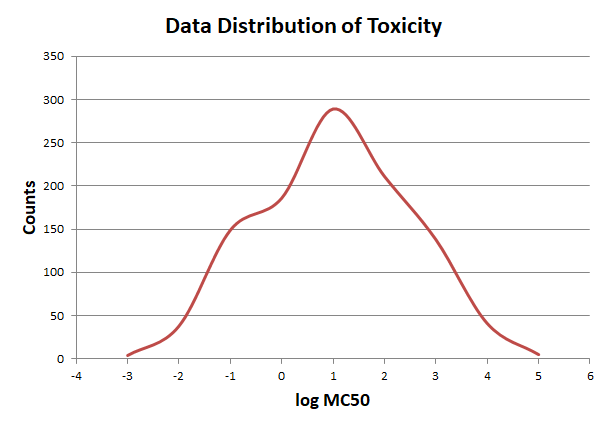
Standardization of score
Graphs below show the distribution of our data.
Fig.4. Gibbs standard energy data distribution.
For each pathway, every reaction r in the pathway has the score log f(r),The score of the pathway is as follows:
\[S = \log f(r1) + \log f(r2) + ... + \log f(rn)\]
(Equation 1.3)
Every reaction r in the pathway has the score log f(r),S refers to total score.S is used to evaluate the pathway. The higher the score is, the better the pathway is.
\[{S_{total}} = \left( {\begin{array}{*{20}{c}}{{S_{\;th}}}&{{S_t}}&{{S_f}}\end{array}} \right)\left( {\begin{array}{*{20}{c}}{{w_{th}}}\\{{w_t}}\\{{w_f}}\end{array}} \right)\]
(Equation 1.4)
The equation above show how the total score is calculated. Corresponding to each ranking criteria, we give them a certain weight.Of course, users can adjust the weight as well. Consequently, the result list is arranged in descending order of total score.
Standardization of score
Graphs below show the distribution of our data.
 In order to elimate the influence of exceptional data, we use pauta criterion to calculate the upper and lower limit according to average value and variance.
\[\begin{array}{l}\mu {\rm{ = }}\frac{1}{n}\sum\limits_{i = 1}^n {arra{y_i}} \\\sigma = \frac{1}{n}\sum\limits_{i = 1}^n {{{(arra{y_i} - \mu )}^2}} \\lower = \mu - 3\sigma \\upper = \mu + 3\sigma \end{array}\]
(Equation 1.5)
\[\begin{array}{l}arra{y_i} = \left\{ \begin{array}{l}lower,{\rm{ }}arra{y_i} < lower\\arra{y_i},{\rm{ }}lower \le arra{y_i} \le upper\\upper,{\rm{ }}arra{y_i} > upper\end{array} \right.\\{\rm{array = }}\left( {array - \mu } \right)/\sigma \end{array}\]
(Equation 1.6)
The distribution of reaction frequency is skewed, cause most reactions can only endogenously construct in a few organisms, which leads to the unbalance of score values. So before turning the frequency data into the standard normal distribution, we use ln(x) to process it to get a more reliable result.We adjust the score array by the limits and turn it into the standard normal distribution. So that all the scores of different criteria are on the same scale, and we can calculate the total score through weighted summation method.
Additional function algorithm
Microorganism recommendation
After searching the pathways, we first select n(n is defined by users) pathways ranking by sum of free Gibbs energy and then use previous scoring method to calculate each route’s score of certain organism. Next we rank the average score of all species and the highest is the best. The number of the selected pathways n can be defined by users. The default value is 50.
In order to elimate the influence of exceptional data, we use pauta criterion to calculate the upper and lower limit according to average value and variance.
\[\begin{array}{l}\mu {\rm{ = }}\frac{1}{n}\sum\limits_{i = 1}^n {arra{y_i}} \\\sigma = \frac{1}{n}\sum\limits_{i = 1}^n {{{(arra{y_i} - \mu )}^2}} \\lower = \mu - 3\sigma \\upper = \mu + 3\sigma \end{array}\]
(Equation 1.5)
\[\begin{array}{l}arra{y_i} = \left\{ \begin{array}{l}lower,{\rm{ }}arra{y_i} < lower\\arra{y_i},{\rm{ }}lower \le arra{y_i} \le upper\\upper,{\rm{ }}arra{y_i} > upper\end{array} \right.\\{\rm{array = }}\left( {array - \mu } \right)/\sigma \end{array}\]
(Equation 1.6)
The distribution of reaction frequency is skewed, cause most reactions can only endogenously construct in a few organisms, which leads to the unbalance of score values. So before turning the frequency data into the standard normal distribution, we use ln(x) to process it to get a more reliable result.We adjust the score array by the limits and turn it into the standard normal distribution. So that all the scores of different criteria are on the same scale, and we can calculate the total score through weighted summation method.
Additional function algorithm
Microorganism recommendation
After searching the pathways, we first select n(n is defined by users) pathways ranking by sum of free Gibbs energy and then use previous scoring method to calculate each route’s score of certain organism. Next we rank the average score of all species and the highest is the best. The number of the selected pathways n can be defined by users. The default value is 50.
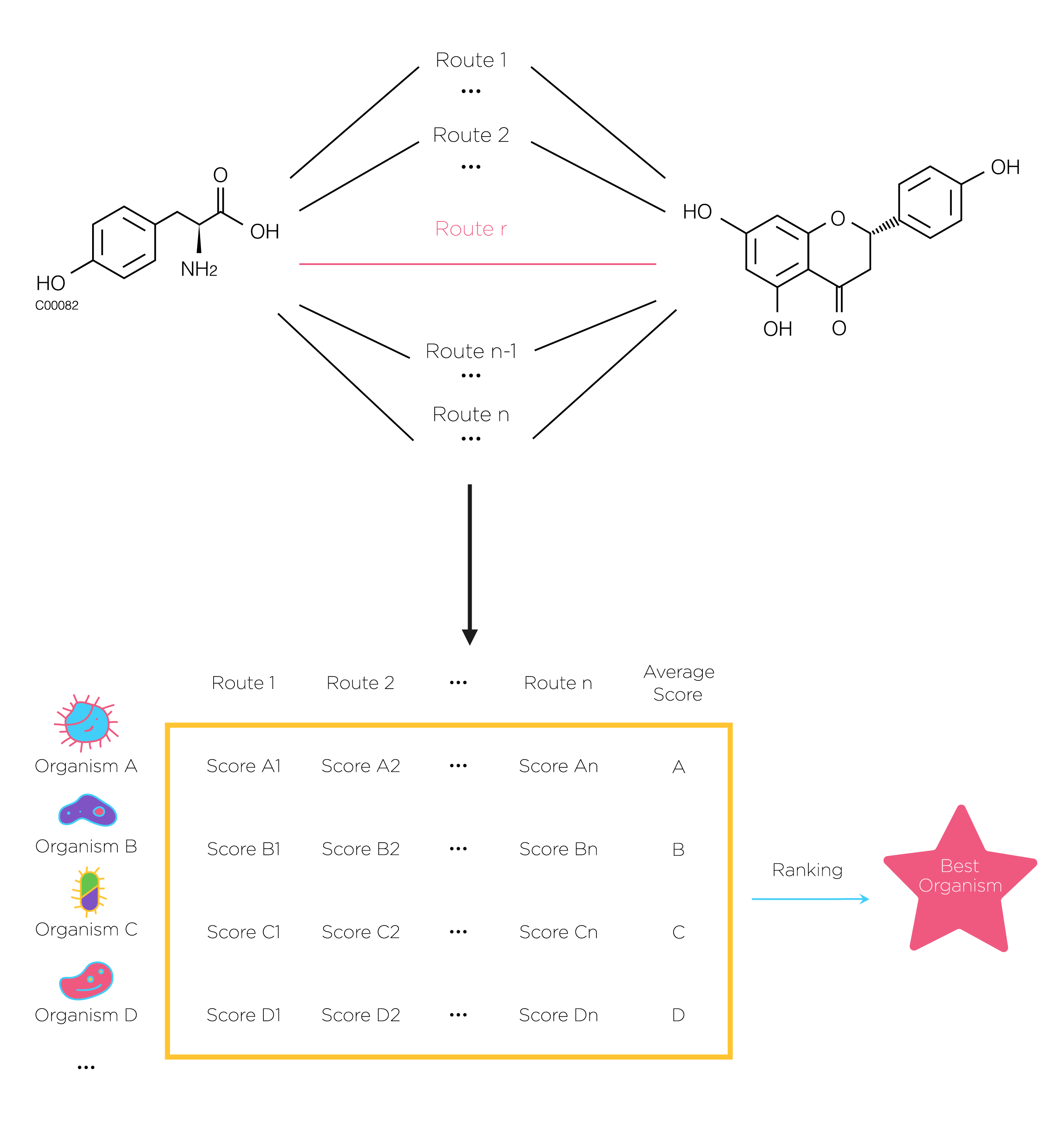 Fig.5. At first, search all possible pathway by using DFS.then use previous scoring method to calculate each route’s score of certain organism. Next we rank the average score of all species and the highest is the best. The number of the selected pathways n can be defined by users.
The average score of every organism:
\[Ave(A) = \frac{{\sum\limits_{i = 1}^n {Score{A_i}} }}{n}\]
(Equation 2.1)
The organism with highest score will be the best.
\[{Max\left\{ {Ave(A),Ave(B),Ave(C),Ave(D)...} \right\}\begin{array}{*{20}{c}}{}&{}\end{array}}\]
(Equation 2.2)
Flux balance analysis(FBA)
Flux balance analysis is a mathematical approach for analyzing the flow of metabolites through a metabolic network. It required very little information in terms of the enzyme kinetic parameters and concentration of metabolites in the system in contrast to the traditionally followed approach of metabolic modeling using coupled ordinary differential equations.[3] FBA achieves this by making two assumptions, steady state and optimality.
Assumption 1: The modeled system has entered a steady state, where the metabolite concentrations no longer change, i.e. in each metabolite node the producing and consuming fluxes cancel each other out.
Assumption 2: The organism has been optimized through evolution for some biological goal, such as optimal growth or conservation of resources.
We use the COBRApy package to implement the function of FBA. [4]The following are illustrations of flux balance analysis.
First we construct a new model based on a model of E. coli core metabolism. This genome-scale metabolic network contains the core metabolism reactions in E. coli. When we need to construct novel reactions into E.coli, we can add the reactions in Systems Biology Markup Language(SBML) which is an XML-based standard format for distributing models supporting for COBRA models through the FBC extension version 2.
Fig.5. At first, search all possible pathway by using DFS.then use previous scoring method to calculate each route’s score of certain organism. Next we rank the average score of all species and the highest is the best. The number of the selected pathways n can be defined by users.
The average score of every organism:
\[Ave(A) = \frac{{\sum\limits_{i = 1}^n {Score{A_i}} }}{n}\]
(Equation 2.1)
The organism with highest score will be the best.
\[{Max\left\{ {Ave(A),Ave(B),Ave(C),Ave(D)...} \right\}\begin{array}{*{20}{c}}{}&{}\end{array}}\]
(Equation 2.2)
Flux balance analysis(FBA)
Flux balance analysis is a mathematical approach for analyzing the flow of metabolites through a metabolic network. It required very little information in terms of the enzyme kinetic parameters and concentration of metabolites in the system in contrast to the traditionally followed approach of metabolic modeling using coupled ordinary differential equations.[3] FBA achieves this by making two assumptions, steady state and optimality.
Assumption 1: The modeled system has entered a steady state, where the metabolite concentrations no longer change, i.e. in each metabolite node the producing and consuming fluxes cancel each other out.
Assumption 2: The organism has been optimized through evolution for some biological goal, such as optimal growth or conservation of resources.
We use the COBRApy package to implement the function of FBA. [4]The following are illustrations of flux balance analysis.
First we construct a new model based on a model of E. coli core metabolism. This genome-scale metabolic network contains the core metabolism reactions in E. coli. When we need to construct novel reactions into E.coli, we can add the reactions in Systems Biology Markup Language(SBML) which is an XML-based standard format for distributing models supporting for COBRA models through the FBC extension version 2.
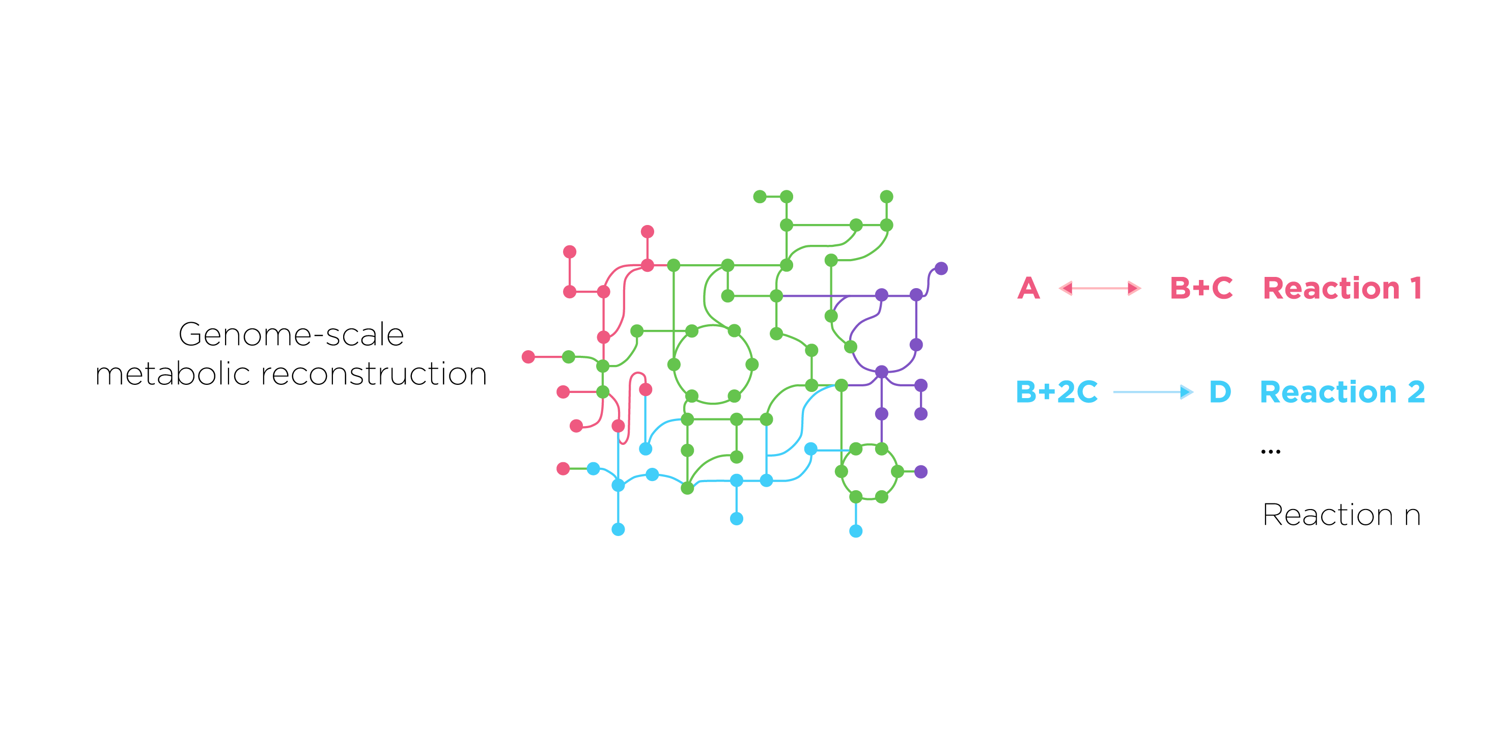
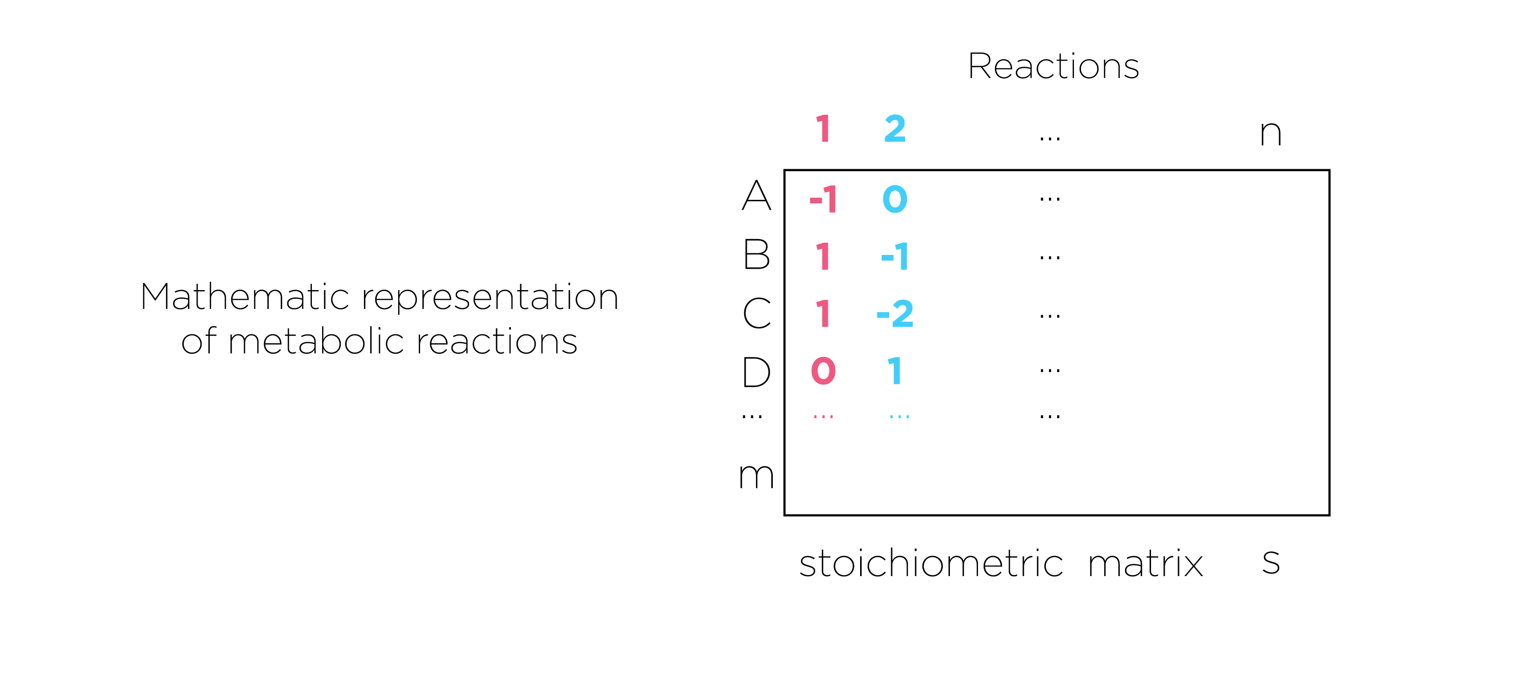 Fig.7.we present metabolic reactions as a stoichiometric matrix (S) of size m × n. Every row of this matrix represents one unique compound (for a system with m compounds) and every column represents one reaction (n reactions).
Constraints are represented in two ways, as equations that present steady-state mass balance and as inequalities that impose bounds on the system.
The concentrations of all metabolites are represented by the vector x, with length m. The flux through all of the reactions in a network is represented by the vector v, which has a length of n. A steady-state mass balance constraint was imposed according to assumption 1.
\[\begin{array}{l}dX/dt = 0\\
{\rm{ }}S \times v = 0\end{array}\]
(Equation 3.1)
Every reaction will be given upper and lower bounds, which define the maximum and minimum allowable fluxes of the reactions. In our software, v_^Upper was set to 1000 mmol/gDW/hour and v_^Lower was set to 0 or -1000 mmol/gDW/hour for irreversible and reversible reactions, respectively.
\[{\rm{ }}{v^{Lower}} \le {v_i} \le {v^{Upper}}\]
(Equation 3.2)
The next step is to define the objective function. It can be any linear combination of fluxes, where c is a vector of weights indicating how much each reaction (such as the biomass reaction when simulating maximum growth) contributes to the objective function. This function is defined by users.
\[Z = {c^T}v\]
(Equation 3.3)
Last we use linear programming to identify a flux distribution that maximizes or minimizes the objective function within the space of allowable fluxes defined by the constraints imposed by the mass balance equations and reaction bounds.
Similarity Comparison of Compound
We use Extended-Connectivity Fingerprints (ECFPs) to present the structure of compound for molecular similarity searching. ECFPs represent molecular structures by means of circular atom neighborhoods.[5]
Representation:
The representation of ECFPs is by means of varying-length lists of integer identifiers. Each identifier represents a particular substructure, more precisely, a circular atom neighborhood, which is present in the molecule. This identifier captures some local information about the corresponding atom in such a way that various atom properties (e.g., atomic number, connection count, etc.) are packed into a single integer value using a hash function. [5]The list of integer identifiers is sorted in ascending order. Then the identifier list is converted to the fixed length bit string.[6]
Fig.7.we present metabolic reactions as a stoichiometric matrix (S) of size m × n. Every row of this matrix represents one unique compound (for a system with m compounds) and every column represents one reaction (n reactions).
Constraints are represented in two ways, as equations that present steady-state mass balance and as inequalities that impose bounds on the system.
The concentrations of all metabolites are represented by the vector x, with length m. The flux through all of the reactions in a network is represented by the vector v, which has a length of n. A steady-state mass balance constraint was imposed according to assumption 1.
\[\begin{array}{l}dX/dt = 0\\
{\rm{ }}S \times v = 0\end{array}\]
(Equation 3.1)
Every reaction will be given upper and lower bounds, which define the maximum and minimum allowable fluxes of the reactions. In our software, v_^Upper was set to 1000 mmol/gDW/hour and v_^Lower was set to 0 or -1000 mmol/gDW/hour for irreversible and reversible reactions, respectively.
\[{\rm{ }}{v^{Lower}} \le {v_i} \le {v^{Upper}}\]
(Equation 3.2)
The next step is to define the objective function. It can be any linear combination of fluxes, where c is a vector of weights indicating how much each reaction (such as the biomass reaction when simulating maximum growth) contributes to the objective function. This function is defined by users.
\[Z = {c^T}v\]
(Equation 3.3)
Last we use linear programming to identify a flux distribution that maximizes or minimizes the objective function within the space of allowable fluxes defined by the constraints imposed by the mass balance equations and reaction bounds.
Similarity Comparison of Compound
We use Extended-Connectivity Fingerprints (ECFPs) to present the structure of compound for molecular similarity searching. ECFPs represent molecular structures by means of circular atom neighborhoods.[5]
Representation:
The representation of ECFPs is by means of varying-length lists of integer identifiers. Each identifier represents a particular substructure, more precisely, a circular atom neighborhood, which is present in the molecule. This identifier captures some local information about the corresponding atom in such a way that various atom properties (e.g., atomic number, connection count, etc.) are packed into a single integer value using a hash function. [5]The list of integer identifiers is sorted in ascending order. Then the identifier list is converted to the fixed length bit string.[6]
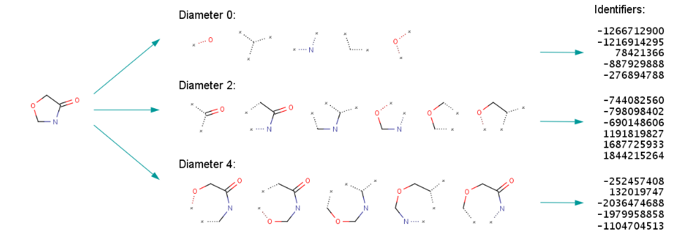 Fig.8. ECFP generation process.
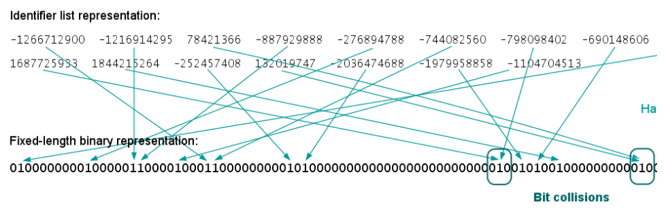 Fig.9. Generation of the fixed-length bit string ("folding")
More information could be found in here.
We turn the fixed-length binary of a compound into an array. We use dice coefficient to evaluate the similarity of two compounds, which is a function to measure the set similarity.
Length: This parameter specifies the length of the bit string representation. The default length is 1024.
a: Array of compound a
b: Array of compound b
\[{\rm{ }}Dice(a,b) = \frac{{2 \times \sum\limits_{i = 1}^{length(a)} {commo{n_i}(a,b)} }}{{length(a) + length(b)}}\]
(Equation 4.1)
\[commo{n_i}(a,b) = \left\{ \begin{array}{l}1,{\rm{ }}\begin{array}{*{20}{c}}{}\end{array}{{\rm{a}}_i} = {b_i}\\0{\rm{, }}\begin{array}{*{20}{c}}{}\end{array}{{\rm{a}}_i} \ne {b_i}\end{array} \right.\]
(Equation 4.2)
Atom conservation
There is a one-to-one correspondence between atom index from reactant and atom index from product in MetaCyc. We integrated the data form into the main pairs in KEGG. We cleaned and removed the redundant data. In one pathway, each step of the reaction is recursive, leaving only the atomic number derived from the source compound, and the rest of the positions are -1. Finally, you can calculate how many atoms in the target are from the source compound.
In order to calculate the final atom conservation rate in a pathway, we need to figure out a data format to describe the atom transferring. In our data format, we create an array for each reactant and product. Every atom in the product has a specific position which is labeled as a sequential array. Each number in the array of reactant means the position of the target compound that atom will transfer to.
Fig.9. Generation of the fixed-length bit string ("folding")
More information could be found in here.
We turn the fixed-length binary of a compound into an array. We use dice coefficient to evaluate the similarity of two compounds, which is a function to measure the set similarity.
Length: This parameter specifies the length of the bit string representation. The default length is 1024.
a: Array of compound a
b: Array of compound b
\[{\rm{ }}Dice(a,b) = \frac{{2 \times \sum\limits_{i = 1}^{length(a)} {commo{n_i}(a,b)} }}{{length(a) + length(b)}}\]
(Equation 4.1)
\[commo{n_i}(a,b) = \left\{ \begin{array}{l}1,{\rm{ }}\begin{array}{*{20}{c}}{}\end{array}{{\rm{a}}_i} = {b_i}\\0{\rm{, }}\begin{array}{*{20}{c}}{}\end{array}{{\rm{a}}_i} \ne {b_i}\end{array} \right.\]
(Equation 4.2)
Atom conservation
There is a one-to-one correspondence between atom index from reactant and atom index from product in MetaCyc. We integrated the data form into the main pairs in KEGG. We cleaned and removed the redundant data. In one pathway, each step of the reaction is recursive, leaving only the atomic number derived from the source compound, and the rest of the positions are -1. Finally, you can calculate how many atoms in the target are from the source compound.
In order to calculate the final atom conservation rate in a pathway, we need to figure out a data format to describe the atom transferring. In our data format, we create an array for each reactant and product. Every atom in the product has a specific position which is labeled as a sequential array. Each number in the array of reactant means the position of the target compound that atom will transfer to.
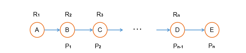 Fig.10. Some concepts we define in a certain pathway.
\[T(i,source,target) = \left\{ \begin{array}{l} - 1{\rm{ , }}\begin{array}{*{20}{c}}{}&{}\end{array}{\rm{ }}{{\rm{i}}^{th}}{\rm{ atom}}\begin{array}{*{20}{c}}{}\end{array}{\rm{of}}\begin{array}{*{20}{c}}{}\end{array}{\rm{source}}\begin{array}{*{20}{c}}{}\end{array}{\rm{doesn't}}\begin{array}{*{20}{c}}{}\end{array}{\rm{transfer}}\begin{array}{*{20}{c}}{}\end{array}{\rm{to}}\begin{array}{*{20}{c}}{}\end{array}{\rm{target}}\\x{\rm{ , }}\begin{array}{*{20}{c}}{}&{}\end{array}{\rm{ }}{{\rm{i}}^{th}}{\rm{ atom}}\begin{array}{*{20}{c}}{}\end{array}{\rm{of}}\begin{array}{*{20}{c}}{}\end{array}{\rm{source}}\begin{array}{*{20}{c}}{}\end{array}{\rm{transfers}}\begin{array}{*{20}{c}}{}\end{array}{\rm{to}}\begin{array}{*{20}{c}}{}\end{array}{\rm{the}}\begin{array}{*{20}{c}}{}\end{array}{{\rm{x}}^{th}}\begin{array}{*{20}{c}}{}\end{array}{\rm{atom}}\begin{array}{*{20}{c}}{}\end{array}{\rm{of}}\begin{array}{*{20}{c}}{}\end{array}{\rm{target}}\end{array} \right.\]
(Equation 5.1)
\[\begin{array}{l}{{\rm{R}}_j}(i) = T(i,{{\rm{R}}_{\rm{j}}}{\rm{,}}{{\rm{P}}_{\rm{j}}}{\rm{) }}\begin{array}{*{20}{c}}{}&{}\end{array}{\rm{ i = 1,2, }}...{\rm{ , A(}}{{\rm{R}}_{\rm{j}}}{\rm{) }}\begin{array}{*{20}{c}}{}&{}\end{array}{\rm{ j = 1,2, }}...{\rm{ , n}}\\{\rm{ }}{{\rm{P}}_j}(i) = T(i,{{\rm{P}}_j}{\rm{,}}{{\rm{R}}_{\rm{j}}}{\rm{) }}\begin{array}{*{20}{c}}{}&{}\end{array}{\rm{ i = 1,2, }}...{\rm{ , A(}}{{\rm{P}}_{\rm{j}}}{\rm{) }}\begin{array}{*{20}{c}}{}&{}\end{array}{\rm{ j = 1,2, }}...{\rm{ , n}}\end{array}\]
(Equation 5.2)
where Rj denotes the nth reactant, Rj(i) denotes the ith number of the Rj array, n denotes the amount of reactants in this pathway, A(Rj) denotes the amount of atoms in Rj. Other symbols with P have the same meanings about product.
\[{{\rm{R}}_{{\rm{j + 1}}}}(i) = \left\{ \begin{array}{l} - 1,\begin{array}{*{20}{c}}{}&{}&{}&{}&{}&{}&{}&{}&{}\end{array}{{\rm{P}}_{\rm{j}}}(i) = - 1\\T(i,{\rm{reactant,product),}}\begin{array}{*{20}{c}}{}&{}\end{array}{{\rm{P}}_{\rm{j}}}(i) \ne - 1\end{array} \right.\]
(Equation 5.3)
Since the jth product is the (j+1)th reactant in the same pathway, the Rj+1 array should be adjusted according to the Pn array. Only the atoms from nth reactant can transfer to the (j+1)th reactant. In this way we can find out how many atoms are conserved through our data format.
\[\begin{array}{l}{\rm{C(}}{{\rm{R}}_{\rm{j}}}(i)) = \left\{ \begin{array}{l}0,{\rm{ }}{{\rm{R}}_{\rm{j}}}(i) = - 1\\1,{\rm{ }}{{\rm{R}}_{\rm{j}}}(i) \ne - 1{\rm{ }}\end{array} \right.\begin{array}{*{20}{c}}{}&{}\end{array}i = 1,2,...,{\rm{ A(}}{{\rm{R}}_{\rm{j}}}{\rm{)}}\\{\rm{ C(}}{{\rm{P}}_{\rm{j}}}(i)) = \left\{ \begin{array}{l}0,{\rm{ }}{{\rm{P}}_{\rm{j}}}(i) = - 1\\1,{\rm{ }}{{\rm{P}}_{\rm{j}}}(i) \ne - 1{\rm{ }}\end{array} \right.\begin{array}{*{20}{c}}{}&{}\end{array}i = 1,2,...,{\rm{ A(}}{{\rm{P}}_{\rm{j}}}{\rm{)}}\end{array}\]
(Equation 5.4)
\[{\rm{ }}Atom\begin{array}{*{20}{c}}{}\end{array}conservation\begin{array}{*{20}{c}}{}\end{array}rate{\rm{ = }}\frac{{\sum\limits_{{\rm{i = 1}}}^{{\rm{A(}}{{\rm{P}}_{\rm{n}}}{\rm{)}}} {{\rm{C(}}{{\rm{P}}_{\rm{n}}}(i))} }}{{{\rm{A}}({R_1})}} \times 100\% \]
(Equation 5.5)
At last, we can calculate the atom conservation rate through the first reactant array and the final product array.
References:
[1] Rogers, D.; Hahn, M. Extended-Connectivity Fingerprints. J. Chem. Inf. Model. 2010, 50(5): 742-754.
[2] Hiroyuki Kuwahara, Meshari Alazmi, Xuefeng Cui and Xin Gao. MRE: a web tool to suggest foreign enzymes for the biosynthesis pathway design with competing endogenous reactions in mind. Nucleic Acids Research, 2016, Vol. 44, Web Server issue W217–W225.
[3] Orth, J.D.; Thiele, I.; Palsson, B.Ø. (2010). "What is flux balance analysis?". Nature Biotechnology. 28: 245–248. doi:10.1038/nbt.1614. PMC 3108565 Freely accessible. PMID 20212490
[4] Schellenberger J, Que R, Fleming RMT, Thiele I, Orth JD, Feist AM, Zielinski DC, Bordbar A, Lewis NE, Rahmanian S et al., Quantitative prediction of cellular metabolism with constraint-based models: the COBRA Toolbox v2.0 Nature Protocol, 2011,6(9):1290-307.
[5] Rogers, D.; Hahn, M. Extended-Connectivity Fingerprints. J. Chem. Inf. Model. 2010, 50(5): 742-754.
[6] Morgan, H. L. The Generation of a Unique Machine Description for Chemical Structures - A Technique Developed at Chemical Abstracts Service. J. Chem. Doc. 1965, 5: 107-112.
Fig.10. Some concepts we define in a certain pathway.
\[T(i,source,target) = \left\{ \begin{array}{l} - 1{\rm{ , }}\begin{array}{*{20}{c}}{}&{}\end{array}{\rm{ }}{{\rm{i}}^{th}}{\rm{ atom}}\begin{array}{*{20}{c}}{}\end{array}{\rm{of}}\begin{array}{*{20}{c}}{}\end{array}{\rm{source}}\begin{array}{*{20}{c}}{}\end{array}{\rm{doesn't}}\begin{array}{*{20}{c}}{}\end{array}{\rm{transfer}}\begin{array}{*{20}{c}}{}\end{array}{\rm{to}}\begin{array}{*{20}{c}}{}\end{array}{\rm{target}}\\x{\rm{ , }}\begin{array}{*{20}{c}}{}&{}\end{array}{\rm{ }}{{\rm{i}}^{th}}{\rm{ atom}}\begin{array}{*{20}{c}}{}\end{array}{\rm{of}}\begin{array}{*{20}{c}}{}\end{array}{\rm{source}}\begin{array}{*{20}{c}}{}\end{array}{\rm{transfers}}\begin{array}{*{20}{c}}{}\end{array}{\rm{to}}\begin{array}{*{20}{c}}{}\end{array}{\rm{the}}\begin{array}{*{20}{c}}{}\end{array}{{\rm{x}}^{th}}\begin{array}{*{20}{c}}{}\end{array}{\rm{atom}}\begin{array}{*{20}{c}}{}\end{array}{\rm{of}}\begin{array}{*{20}{c}}{}\end{array}{\rm{target}}\end{array} \right.\]
(Equation 5.1)
\[\begin{array}{l}{{\rm{R}}_j}(i) = T(i,{{\rm{R}}_{\rm{j}}}{\rm{,}}{{\rm{P}}_{\rm{j}}}{\rm{) }}\begin{array}{*{20}{c}}{}&{}\end{array}{\rm{ i = 1,2, }}...{\rm{ , A(}}{{\rm{R}}_{\rm{j}}}{\rm{) }}\begin{array}{*{20}{c}}{}&{}\end{array}{\rm{ j = 1,2, }}...{\rm{ , n}}\\{\rm{ }}{{\rm{P}}_j}(i) = T(i,{{\rm{P}}_j}{\rm{,}}{{\rm{R}}_{\rm{j}}}{\rm{) }}\begin{array}{*{20}{c}}{}&{}\end{array}{\rm{ i = 1,2, }}...{\rm{ , A(}}{{\rm{P}}_{\rm{j}}}{\rm{) }}\begin{array}{*{20}{c}}{}&{}\end{array}{\rm{ j = 1,2, }}...{\rm{ , n}}\end{array}\]
(Equation 5.2)
where Rj denotes the nth reactant, Rj(i) denotes the ith number of the Rj array, n denotes the amount of reactants in this pathway, A(Rj) denotes the amount of atoms in Rj. Other symbols with P have the same meanings about product.
\[{{\rm{R}}_{{\rm{j + 1}}}}(i) = \left\{ \begin{array}{l} - 1,\begin{array}{*{20}{c}}{}&{}&{}&{}&{}&{}&{}&{}&{}\end{array}{{\rm{P}}_{\rm{j}}}(i) = - 1\\T(i,{\rm{reactant,product),}}\begin{array}{*{20}{c}}{}&{}\end{array}{{\rm{P}}_{\rm{j}}}(i) \ne - 1\end{array} \right.\]
(Equation 5.3)
Since the jth product is the (j+1)th reactant in the same pathway, the Rj+1 array should be adjusted according to the Pn array. Only the atoms from nth reactant can transfer to the (j+1)th reactant. In this way we can find out how many atoms are conserved through our data format.
\[\begin{array}{l}{\rm{C(}}{{\rm{R}}_{\rm{j}}}(i)) = \left\{ \begin{array}{l}0,{\rm{ }}{{\rm{R}}_{\rm{j}}}(i) = - 1\\1,{\rm{ }}{{\rm{R}}_{\rm{j}}}(i) \ne - 1{\rm{ }}\end{array} \right.\begin{array}{*{20}{c}}{}&{}\end{array}i = 1,2,...,{\rm{ A(}}{{\rm{R}}_{\rm{j}}}{\rm{)}}\\{\rm{ C(}}{{\rm{P}}_{\rm{j}}}(i)) = \left\{ \begin{array}{l}0,{\rm{ }}{{\rm{P}}_{\rm{j}}}(i) = - 1\\1,{\rm{ }}{{\rm{P}}_{\rm{j}}}(i) \ne - 1{\rm{ }}\end{array} \right.\begin{array}{*{20}{c}}{}&{}\end{array}i = 1,2,...,{\rm{ A(}}{{\rm{P}}_{\rm{j}}}{\rm{)}}\end{array}\]
(Equation 5.4)
\[{\rm{ }}Atom\begin{array}{*{20}{c}}{}\end{array}conservation\begin{array}{*{20}{c}}{}\end{array}rate{\rm{ = }}\frac{{\sum\limits_{{\rm{i = 1}}}^{{\rm{A(}}{{\rm{P}}_{\rm{n}}}{\rm{)}}} {{\rm{C(}}{{\rm{P}}_{\rm{n}}}(i))} }}{{{\rm{A}}({R_1})}} \times 100\% \]
(Equation 5.5)
At last, we can calculate the atom conservation rate through the first reactant array and the final product array.
References:
[1] Rogers, D.; Hahn, M. Extended-Connectivity Fingerprints. J. Chem. Inf. Model. 2010, 50(5): 742-754.
[2] Hiroyuki Kuwahara, Meshari Alazmi, Xuefeng Cui and Xin Gao. MRE: a web tool to suggest foreign enzymes for the biosynthesis pathway design with competing endogenous reactions in mind. Nucleic Acids Research, 2016, Vol. 44, Web Server issue W217–W225.
[3] Orth, J.D.; Thiele, I.; Palsson, B.Ø. (2010). "What is flux balance analysis?". Nature Biotechnology. 28: 245–248. doi:10.1038/nbt.1614. PMC 3108565 Freely accessible. PMID 20212490
[4] Schellenberger J, Que R, Fleming RMT, Thiele I, Orth JD, Feist AM, Zielinski DC, Bordbar A, Lewis NE, Rahmanian S et al., Quantitative prediction of cellular metabolism with constraint-based models: the COBRA Toolbox v2.0 Nature Protocol, 2011,6(9):1290-307.
[5] Rogers, D.; Hahn, M. Extended-Connectivity Fingerprints. J. Chem. Inf. Model. 2010, 50(5): 742-754.
[6] Morgan, H. L. The Generation of a Unique Machine Description for Chemical Structures - A Technique Developed at Chemical Abstracts Service. J. Chem. Doc. 1965, 5: 107-112.