It is also a good rule not to put too much confidence in
experimental results until they have been confirmed by
Theory.
-- Sir Arthur Eddington
With our model, we want to join a new generation of interdisciplinarity scientists working at, and exploring on the boundaries of what synthetic biology can deliver. With time nowadays being more precious than ever, we centred our project around saving it, streamlining processes and making these advances accessible to the research community.
We accelerated processes in many regards, but the most efficient way to save time is to know beforehand which experiments to conduct. The predictive powers needed for that can be harnessed by computer-based modelling. We harvested this prediction power with two independent modeling approaches, one predicting the metabolism of Vibrio Natriegens and the other designing an enzyme capable of a novel reaction, decarboxylating malate to 3-hydroxypropionic acid (3HPA).
Metabolic Model
In order to be able to fine-tune synthetic pathways and utilize the well-characterized parts of our cloning toolbox to its fullest potential, we need a model which gives useful predictions of metabolic fluxes. There exists a multitude of approaches to model fluxes – some are on the genomic scale some occupied only with the mechanism of a single enzyme. We have chosen to utilize two different approaches – on one scale we use reaction kinetics to analyze the behavior/kinetics of our inserted enzymes within the metabolism – on the other we use a novel approach called 2S-MFA [Reference] to get a genome-scale perspective on the metabolic fluxes. Using the thereby consolidated theoretical knowledge we can complete the Design-Build-Test-Learn cycle for our metabolic engineering project and use it to iteratively improve our project. With the prediction power of this models, we not only save a lot of time in the lab but we manage to improve the efficiency and productivity, the skill ceiling of our pathway.
Structural model

The pathway we used for production of 3HPA (for details see the description part of the metabolic engineering subgroup) has been explored previously and is based on a combination of known reactions and known enzymes. Combination of different enzymes to make a synthetic pathway is a well-established method in the field of metabolic engineering, but limited to existing reactions and known enzymes. With our structural model, we tried to build a new energetically more favorable pathway which was previously impossible. To accomplish that, we needed to implement a reaction with no known enzyme to catalyse it, the decarboxylation reaction of malate to 3HPA. To build this pathway we decided to engineer an enzyme capable of catalysing this reaction. We investigated the enzyme family of Carboxy-lyases and developed an idea on how to build a binding pocket catalysing this reaction. To evaluate if our binding pocket works, we performed electronic structure calculations. With that, we were able to calculate the activation barrier of the reaction and therefore evaluate if it is possible for the reaction to take place. To advance from a binding pocket to a full enzyme we evaluated in silico mutated versions of acetolactate decarboxylase (ALD). For evaluating which mutants perform best we used MD simulations and checked how well the binding pocket assumed in the electronic structure calculations is represented in the simulations. With the help of these in silico approaches we chose a mutant and tested it in the wetlab.
Teach the rabbit to quack
Expanding the scope of metabolic engineering through novel enzyme engineering
Infrastructure
We want to thank Prof. Kolb and Prof. Klebe for kindly providing us with the necessary infrastructure and software access to perform our calculations. We also want to thank the Marc-2 and the HRZ for the computational resources. For our QM calculations, we used the program GAUSSIAN09 and Chemcraft to set up our systems. For a foray to how these kinds of calculations work, please click below.
Foray to QM Calculations
QM Calculations are the pinnacle of precision compared to all other methods used for calculating molecular systems, but this precision comes with very high computational costs.
All QM calculation try to solve the Schroedinger Equation :

They do that by calculating the Hamiltonian of the system.
The Hamiltonian is an operator that if applied to the wavefunction of a system results in the same wavefunction times its energy.
QM calculations are characterized by two important things: the functional and the basis set used.
The functional is characterized by the way the Hamiltonian is calculated.
For all calculations that we do, we also need a starting point to describe orbitals or the density function (we will go into more detail to this later) and the basis set describes the number and type of the orbital functions that we use to calculate the system.
Born Oppenheimer Approximation
A necessary assumption to use QM methods is the Born Oppenheimer Approximation. This is the approximation that due to the vast difference in speed between the electrons and the nucleus of the atoms the movement of both can be investigated apart from each other. For QM Methods this means that we only look at the movement of electrons and neglect the very slow movements of the nuclei when solving the Schroedinger Equation.
Functionals and Basis sets
Functionals
There are two fundamentally different types of functionals, wave function based and density function based methods.
We only used density function based methods, to be precise B3LYP.
Density Function Theory (DFT) is centered not on the wavefunction but on the square of the wave function, i.e. the electron density.
It is based on the theorem of Hohenberg and Kohn and modern DFT is also based on the Kohn Sham approach.
The electron density is a measurable quantity that is dependent on the cartesian coordinates of the electrons.
In the first days of DFT (when invented by physicists) mostly the Linear Density Approach (LDA) was used and this approach works fine for metallic solids, in which the electrons are evenly distributed.
However, this is a poor approximation when we want to model molecular systems.
As a further Development of this approximation, Gradient corrected methods (GGA) have been invented.
These methods consider the electron density not to be uniform.
There are multiple terms in the Hamiltonian that have to be calculated.
The most troublesome one is the so-called "Exchange-Correlation" term.
There is a class of DFT functionals, the so-called Hybrid Functionals, that use a combination of exchange-correlation terms of different methods.
The method we used, B3LYP, uses a combination of LDA, GGA, and Hartree Fock (A wavefunction based method) exchange-correlation.
Basis Sets
Now that we know which method we use we can take a look at the second important characteristic of our QM calculations, the basis set. All methods described previously, even if based on DFT, use Orbitals in their calculations. By combining a certain number of orbitals the molecular orbitals of the system have to be expressed. This starting number of orbitals is called the basis set. Obviously, the more orbitals we have the more accurate the calculations become, but they also get more demanding. As a small basis set we used the 6-31g* variant and as a bigger basis set, we used cc-pVDZ. In a perfect scenario, the use of a bigger basis set should only improve the accuracy of the result, but it is possible that using a different basis set yields completely different results.
Summary
- Based on Quantum Mechanics
- All electrons investigated
- Bond cleavage and formation can be calculated
- Slow Calculations and limited to small Systems
Foray to Molecular Mechanics
Molecular Mechanics (MM ) uses the laws of classical mechanics to model molecular systems. It can be used to calculate anything ranging between small molecules to big proteins. Each atom is simulated as one single particle, with a radius and charge. Bonded interactions are treated by the famous Hooke's law (i.e. they are springs). This approximation allows us to simulate very big systems, but it is very important to asses which properties we can simulate correctly and therefore investigate. Because classical Molecular Dynamics (MD) Simulations are based on MM , we cannot simulate bond breaking or bond formation which also means that protonation states cannot change during simulation.
Force Fields
To calculate inter- and intramolecular interactions, so-called force fields are used.
With these FF all of these interactions are reduced to single additive terms.
It consists of terms for bond stretching, angle bending, torsions, Lennard-Jones potential (for Van-der-Waals interactions) and electrostatic potential.
It is necessary to parametrize these terms very carefully and this is done by using experimental data or QM calculations.
There are many FF available and we used a force field from the AMBER family called ff14SB (Maier et al.2015).
The complete potential function is given in the following equation:

Kinetic Energy and Time Evolution of a molecular system
If we would just apply all of the physical principles and assumptions mentioned previously, we would minimize the system to the closest potential energy minimum.
For the system to overcome potential energy barriers given by the FF, we have to introduce kinetic energy.
The kinetic energy of all particles in the system is dependent on their temperature and given by a Maxwell-Boltzmann velocity distribution function.

This distribution function contains the kinetic energy of a particle, which is expressed as its momentum.

The total energy of the system is given as the sum of the potential energy (given by the force field) and the kinetic energy.
Each particle in every MD timestep that we investigate has, therefore, three positional coordinates, three momentum coordinates, and a corresponding total energy.

To now introduce time evolution in the system we use classical mechanics and newtons laws of motion in combination with the kinetic energies introduced previously.

To further reduce the computational cost a so-called leapfrog algorithm is used.
As mentioned previously, every particle in the system is described using three positional coordinates, three momentum coordinates, and its corresponding energy.
With the leapfrog algorithm for each step of the MD we only calculate either the positinal coordinates or the momentum coordinates and "leap over" the other.
Periodic Box
MD Simulations are performed within a confined volume, called a unit cell.
This unit cell contains all particles that we simulate (i.e. protein, water, ligand).
This introduces the problem of boundary effects because atoms and molecules close to these boundaries of the unit cell have fewer interaction partners than those in the middle of it.
To avoid boundary effects at the edges of the unit cell we repeat the unit cell periodically.
Thus, the shape of the unit cell has to allow such that a regular space filling lattice of unit cells can be arranged.
In our study, we used a truncated octahedron.
Summary
- Based on Classical Physics
- No Electrons investigated
- No Bond cleavage or formation
- Fast Calculations and big Systems
Motivation
We went to great lengths to develop a workflow for metabolic engineering that utilizes the power of directed evolution and is worthy of synthetic biology in the not so early 21st century. With the very recent Nobel Prize in chemistry towards directed evolution we think we have struck a nerve, and with Vibrio Natriegens this process can be streamlined even further. Traditional Chemistry with Synthesis as its supreme discipline and its implications in the industry is one of the driving forces behind the modern wealth and is being improved on a daily basis. Synthetic Biology and in particular metabolic engineering as a chemical producing science can use that well-established knowledge and expand on it. Due to the completely different approach to synthesizing chemicals, we can mend the problems that classical organic chemistry is facing (e.g. natural products with many stereocenters, necessary purification of products after most reaction steps) and create compounds previously not synthesizable (e.g. Artemisinic acid) or ones that were too costly. Using metabolic engineering also has the advantage to produce chemicals out of renewable resources while many chemicals right now are synthesized starting with fossil oil. To further improve this opportunity to make more of the chemical space synthesizable in a cheap, easy and renewable manner we need to go beyond "mix and match" pathways and explore novel enzymatic reactions. According to (Erb et al.2017) metabolic engineering has been categorized in 5 different levels, depending on the methods employed. These levels and the corresponding metabolic space is displayed in Figure 1. We tried to expand on what we already did in our metabolic engineering project and tap the huge advantages using novel pathways offer. We tried to enable a novel pathway by engineering an enzyme to catalyse a new reaction which corresponds to the 4th level of metabolic engineering.

Design of the binding pocket
The pathway we chose for our metabolic engineering efforts was - in our opinion - the best pathway that has been explored previously. But there are much more possible theoretical (Valdehuesa et al,2013) pathways with remarkable properties that have not been explored yet. The reason is most of the times that it involves one or more reactions with no known enzyme to catalyse them. One theoretical pathway is from a free energy standpoint much more favorable, but there is one step without a known enzyme to catalyse it. We performed an intense literature research and decided to build an enzyme capable of decarboxylating malate to 3HPA. Even with Vibrio natriegens if we would engineer an enzyme to catalyse the wanted reaction using random mutagenesis it would take ages if it succeeds at all. That is why we decided to use a combination of in silico as well as wet lab methods to boost our chances of succeeding.
The pathway that we plan to enable is displayed in Figure 2. The step that has to be catalysed is the decarboxylation reaction of malate to our final product, 3HPA. As a starting point, we investigated the enzyme family of Carboxy-lyases (EC Number 4.1.1). We - in accordance with literature - were not able to find an enzyme that can catalyse this reaction.
However, there were some that we thought could help us to develop a binding pocket capable of decarboxylating malate.
One of those was acetolactate decarboxylase (ALD 4.1.1.5).
The important difference from its natural substrate to malate being that there is a carboxy group in β position (see Figure 4).
In this enzyme with the help of this carboxy group a double bond is formed to an intermediate product (see Figure 4) that we cannot form with malate as substrate. But the zinc cation that is used as a cofactor should be able to bind to malate in a similar way as it does with the natural substrate.
This could be a promising starting point because we would be able to sustain a specific conformation of the substrate and alter the electronic structure of the substrate at the same time.
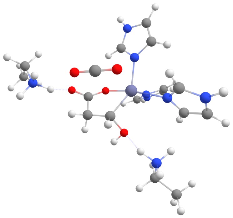
The complex of malate inside the ALD binding pocket is shown in Figure 3.
The zinc cofactor is bound by three histidines and the zinc binds to the malate (or the substrate analog in the real crystal structure) with three interactions.
There is another important residue close to this complex, Arg145.
After the double bond and with it the intermediate product is formed, this residue is protonating the intermediate to form the product.

Another enzyme with an enzyme mechanism that might help us to find a way to catalyse this reaction is Orotidine 5'-phosphate decarboxylase (ODCase 4.1.1.23).
The reaction ODCase catalyses compared to the reaction of ALD and the one we want to catalyse is shown in Figure 4.
In one study conducted by (Courtney et al.2007) using
QM/MM
MD
simulations, the decarboxylation mechanism of ODCase has been investigated.
They have proposed a direct decarboxylation mechanism and calculated a free energy activation barrier that is in good agreement with experimentally obtained values.
The reaction is split into two steps, first the decarboxylation and a simultaneous salt bridge between a lysine and the resulting carbanion.
After this, the lysine protonates the carbanion to yield the final product.
The most important difference between the substrate of ODCase and malate is, that the carbanion stabilized (Figure 4) in the former one whilst there is nearly no stabilization in the latter one.
The idea of our enzyme design is that we use the direct decarboxylation of ODCase and stabilize the carbanion with the cofactor of ALD.
With this plan, we need to engineer the pocket in a way that a lysine side chain can get to the C2-carbon of malate (see Figure 5 for numbering) that shall be protonated.

As a starting point, we looked at all single point mutations to lysine that can be done where the protonated nitrogen of lysine has the possibility to get as close to the malate since this is required for reprotonation. All Mutations investigated are displayed in Table 1.
In the natural binding pocket of ALD there is an arginine residue that is used for reprotonation of the natural substrate.
Because of the possibility that this disturbs the lysine we mutated it in each binding pocket where it is not already mutated to a glycine.
| L34K | G57K | T58K | L62K |
|---|---|---|---|
| E65K | G64K | R145K | V147K |
in silico enzyme design
We developed a double modeling approach to investigate the whole system. First, we investigated the reaction using quantum mechanical calculations (QM) and model the best possible system. Then we control how well this system is retained if we make certain mutations in the ALD with the help of molecular dynamic (MD ) Simulations.
Quantum mechanics calculations
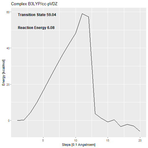
First, we modeled the reaction that we plan to catalyse using QM level calculations. We used density functional theory based method b3-lyp with different basis sets. With these calculations, we tried to get a further insight into the reaction coordinate and all corresponding energies, most importantly the activation energy of the reaction. The activation energy can be calculated as the difference between the energy of the starting compounds and the transition state energy. The activation energy is crucial for the activity of the final enzyme and high activation energies correspond to low or no activity of the final enzyme. According to (Courtney et al.2007) the reaction is split into two steps. First, the decarboxylation happens and a salt bridge is formed between the positively charged lysine and negatively charged carbanion. In a second step one of the protons of the lysine is protonating the negatively charged carbanion and with that the reaction is complete. The first step of the reaction is the rate-limiting step of the reaction (Courtney et al.2007) and because of this, we decided to focus on it.
Building of binding pockets
As a starting point we used the ALD crystal structure of (Marlow et al.2013) (PDB CODE 4BT3). From that, we extracted the position of the three zinc coordinating histidines, the zinc cation, and the substrate and changed the substrate analog ((2R,3R)-2,3-Dihydroxy-2-methylbutanoic acid) to malate. We then built multiple different binding pockets that are displayed in Table [2].
| Type of Binding Pocket | Abbreviation used in Graphs | Residues/Molecules involved |
|---|---|---|
| Binding Pocket without Cofactor | Complex | Lysine, Substrate |
| Binding Pocket | Nor_1 | Three Histidines, Zinc cation, Lysine, Glutamate, Substrate |
| Binding Pocket pre-optimized | Nor_2 | Three Histidines, Zinc cation, Lysine, Glutamate, Substrate |
| Minimal Binding Pocket | Min | Three Histidines, Zinc cation, Lysine, Substrate |
| Binding Pocket with two lysine residues | 2ly | Three Histidines, Zinc cation, Lysine, Lysine, Substrate |
Because we want to resemble the binding pocket to the best of our knowledge we made a system in which we kept Glu253 and added a lysine close to the C2-carbon that it should protonate.
Later we used a pre-optimized structure of previous calculations and used this pre-optimized structure to build a minimal binding pocket where we removed Glu.
We also made one system with two lysine residues.
We will go into detail on why and how we designed this system when we explain the hypothesis.
As a start point, we also used a structure of malate and lysine, referred to as complex in Table 2.
The final systems are displayed in Figure 6.
 a
a b
b c
c d
d
Results of QM Calculations
 a
a b
b c
c d
d
The calculated activation barrier for the complex (cc-pVDZ basis set) is 59.04 kcal/mol [Figure 7a].
This is far over the free energy barrier of ODCase in the literature (15.54 kcal/mol (Courtney et al.2007)).
The addition of the zinc complex that shall stabilize the carbanion (53.48 kcal/mol) [Figure 7c] only benefits the reaction with around 6 kcal/mol.
The transition states that we calculate are confirmed using frequency calculations.
If there is just one negative frequency calculated for an optimized structure, this means that it is a transition state.
The frequency can then be animated, to show the movement that is enforced by it.
An animation of the negative frequency of the minimal binding pocket transition state can be seen in Figure 8.
This was boosting our hope that if we introduce the correct changes to the binding pocket, we could change the electronic structure of malate in a way to sufficiently reduce the activation barrier.
To use this knowledge we set up another system with two lysine residues, one interacting with both carboxy moieties (lys1) and one that shall protonate the C2-carbon (lys2).
The activation barrier (2lys 631g*) was slightly lower than before (~ 43 kcal/mol), but lys2 was not reprotonating the carbanion but interacting with the hydroxy moiety.
Even more interesting was the fact that the carbanion formed a covalent bond with the zinc cation with ca. 10 kcal/mol less energy than the transition state.
The optimized structure with the covalent bond between the zinc cation and the malate is displayed in Figure 9.
Molecular Dynamic (MD ) Simulations
To evaluate how well the system that we tried to engineer in the QM calculations is represented in the complete enzyme systems we performed MD simulations with in silico mutated enzyme versions. We performed 200 ns MD Simulations of all previously mentioned mutated systems as well as the wild-type enzyme with 3 replicas each. With the help of these MD simulations, we are able to evaluate how well the different mutations resemble the system that we designed for the QM calculations.
Setup of MD Simulations
For the MD simulations, we used the ALD crystal structure of [Reference] (PDB CODE 4BT3). We changed the substrate to malate and made the corresponding mutations for each system. Then we capped the termini of the enzyme, checked for missing residues and protonated all residues according to pH 7.0. We visually inspected the residues close to the binding pocket to make sure that all protonation states are correctly assigned. For a more detailed description of our preparation protocol please click below.
In the following, all minimization steps are carried out using pmemd and all MD runs are carried out using pmemd.cuda from the AMBER 16 package. Before the MD run is started, we first heat and equilibrate the system. For that, we minimize the system first with fixed solute heavy atoms and afterwards with constrained solute heavy atoms. The system is annealed to 300K within 25 ps. After that, the density is equilibrated to approximately 1g/ml within 25 ps while lowering the constraints on the solute heavy atoms. A final 5 ns equilibration with fixed volume and temperature is carried out before starting the productive MD.
Results of MD Simulations
We previously established the mutations we introduced in silico (Table 1) to ALD.
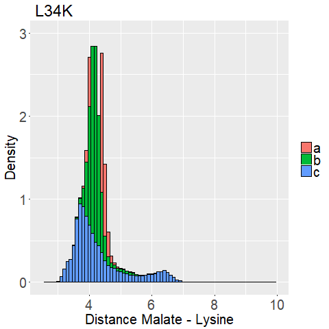
For evaluating how well the mutants resemble the binding pocket developed with the help of the QM we developed a mechanical descriptor.
The distance between the binding pockets lysine side chain and the malate is used.
We measured the distance between the lysine sidechains nitrogen atom and the C2-carbon that should be protonated of the malate for every frame of every MD Simulation.
This way we can evaluate if the lysine is close enough to the C2-Carbon for reprotonation as well as interaction with the carboxy moieties.
An animation of one MD Simulation (L34K Replica 1) with the distance highlighted is shown in Figure 10.
 a
a b
b c
c d
d e
e f
f
This is very promising because it means that there is not only one potential position to introduce point mutations, which opens up further possibilities for enzyme design.
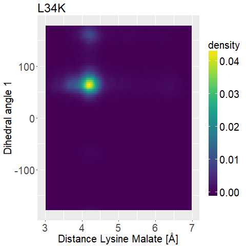
To further distinguish between the different variations we decided to look at two dihedral angles of the lysine sidechain to evaluate its flexibility.
To display this we used two-dimensional histograms.
The 2d histograms we developed contain all the information the 1d histograms had.
However, they do not "just" count how many instances of an investigation we have in a bin, but rather how many combinations of investigations we have in a small two-dimensional box.
This way we can not only investigate which distances each mutated enzyme has, but also pair this together with the corresponding dihedral angle(s).
We also use normalized 2d-histograms, which means that the total area of the 2d-histogram is normalized to one.
What we are looking for is a mutated enzyme which consistently shows low lysine-malate distances while simultaneously showing some flexibility in the dihedral angles.
If the side chain of lysine shows too much flexibility (i.e. Figure 13d), the sidechains stability at the correct position is unfavorable.
A ligand that shows too low flexibility (i.e. Figure 12b) the position is entropically unbeneficial.
The results are displayed in Figure 12 and 13.
 a
a b
b c
c d
d e
e f
f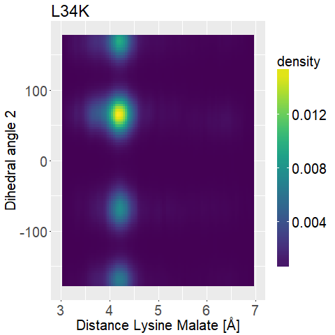 a
a b
b c
c d
d e
e f
fWe can observe high densities for R145K (Figure 12b), which means that the single state it is in is also very stable. The very stable dihedral angles indicate an entropically unbeneficial conformation of the side chain. For T58K we observe a stable conformation at a low distance, but also that it is stable at a broad range of distances. L34K has multiple stable angles for dihedral angle 2, whilst having only one for dihedral angle 1 and a small and low distance range. If we take the 1d as well as the 2d histograms into account, L34K seems to be the most promising of all of the different mutated enzymes.
Wetlab
Summary
We have developed an in silico workflow to design a novel decarboxylase that with minor changes can be adapted for other carbon-carbon bond cleavage enzyme designs, de novo or not. We predicted that the activation barrier for the reaction is too high for successful catalysis. Because of time and resources we were only able to look at single point and double mutations, but the reduction in the activation barrier when using lysine to interact with the carboxy functions showed that there are possibilities to change the electronic structure of the substrate. With the covalent bond between the zinc cation and the substrate we also showed that we can and should dare to think outside the box to find novel ways that could help to create a novel enzyme mechanism. With the data obtained through our MD Simulations we showed that there are multiple positions in the binding pocket of ALD where we can introduce point mutations that interact with the substrate.
Outlook
The next in silico steps are further exploring the possibilities of multiple mutations (and therefore multiple sidechains in the binding pocket). We have shown that the interaction of charged side chains, in our case lysine, can lower the activation energy. We think multiple sidechains with the possibility of building salt bridges or hydrogen bonds with malate will alter the electronic structure even further. We have also shown that the nor_1 system (with zinc cation) has only an about ~6kcal/mol smaller activation barrier than the complex (without zinc cation). Even though the zinc cofactor offers the opportunity to stabilize malate in the binding pocket in a very specific conformation it is probably worthwhile to investigate a more ODCase style binding pocket without a cofactor. ODCase speeds the reaction of the natural substrate up by a factor of 10^17 without a cofactor and is a fascinating enzyme because of that. We strongly believe that there is a possibility to design a binding pocket capable to catalyse this reaction using a ODCase style binding pocket. We do not need to engineer an enzyme capable of such a reaction speedup as in ODCase, it is fully sufficient to make an enzyme that is capable to catalyse measurable quantities and improve it using our metabolic engineering workflow. Due to the vast differences between the substrates the binding pocket of ODCase is too big for Malate. The binding pocket could only be utilized for malate if we would introduce multiple changes and maybe the backbone of the protein is not suited to design the functioning, yet unknown binding pocket. It is possible to design a binding pocket without cofactor using the method we established and to design an enzyme starting from the binding pocket we could either engineer ODCase or use a programm like Rosetta to screen for other possible candidates with fitting binding pockets."I have not failed. I've just found 10.000 ways that won't work." - Thomas A. Edison
Overall, even though we were not able to design a working enzyme, we are very optimistic about the prospect of it in the future and think that our results can function as a fundament that others can build on.