Team:NCTU Formosa/Dry Lab/Productivity Model

MENU

HOME

TEAM

Team

PROJECT

PARTS

HUMAN PRACTICES

AWARDS

Navigation Bar

☰

Project

Dry Lab

Microbiota Prediction

Wet Lab

Parts

Human Practice

Education and Public Engagement

Team

Notebook

Productivity Model

The core nutrients nitrogen, phosphorus and potassium directly impact the productivity of crops. To predict how our fertilizers affect crop yield, we generate a model that relates cumulative N, P and K application to final curcumin concentration. Using neural networks is a popular method of deriving connection between a combination of factors and a final value, in this case a combination of N, P and K values and a productivity value. Constructing the following neural network with back-propagating methods results in a non-linear regression model that predicts productivity from cumulative fertilization.

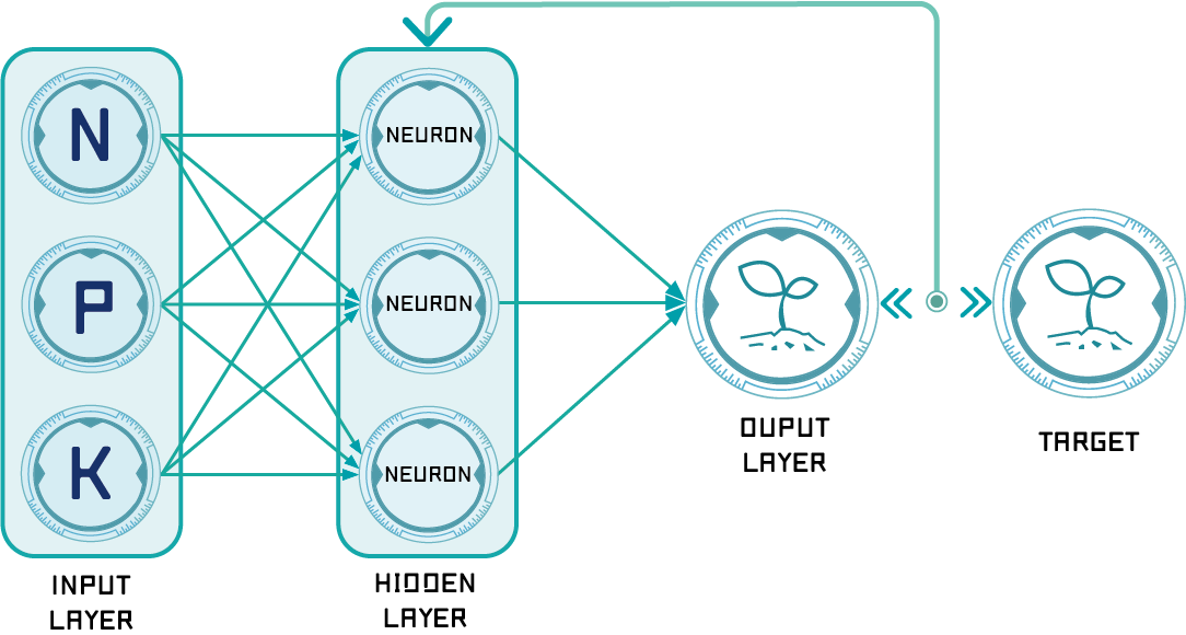
Figure 1: Schema of the neural network

We use simple three layer ANN (Artificial Neural Network) design to build up our productivity model, including one input layer, one hidden layer, and one output layer. Input layer contains the data of nitrogen, phosphate, and potassium, three nutrients added to soil respectively. Hidden layer contains three neuron (more details will be explained below). Finally, output layer contains one predicted productivity.

ANN Training Process

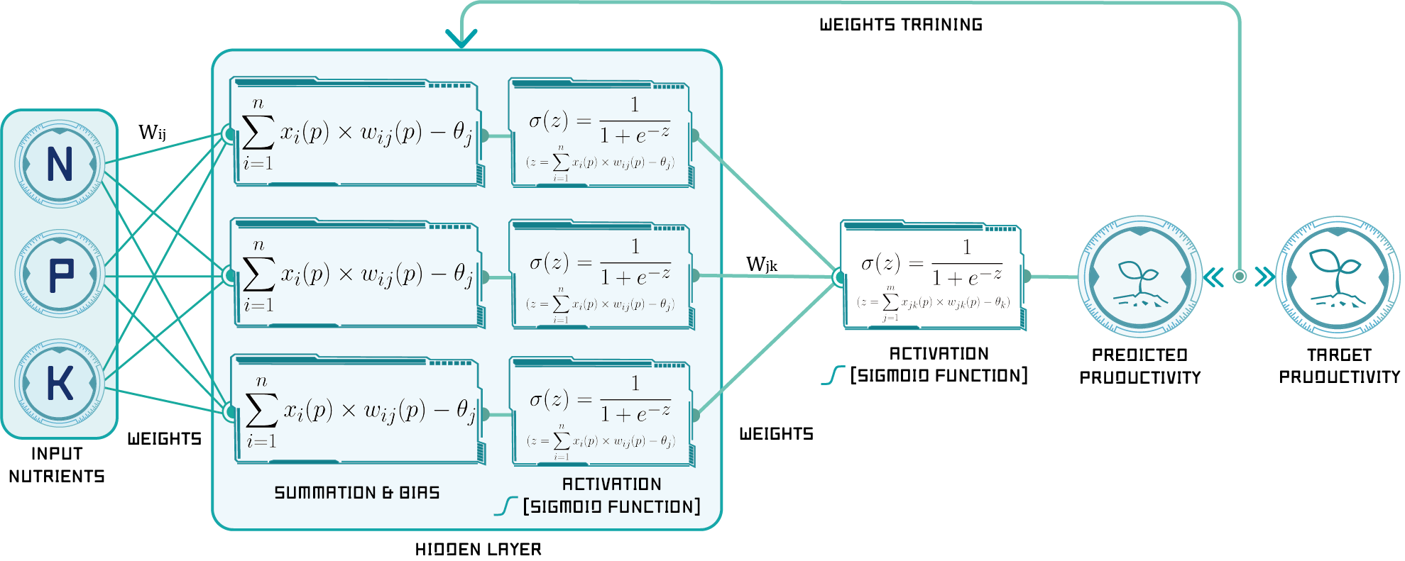
Figure 2: The detail of the neural network training process

1. Initialization

Set all the weights and threshold levels of the network to random numbers uniformly distributed inside a small range (Haykin, 2008): $$\left ( -\frac{1}{Fi},+\frac{1}{Fi} \right )$$ where Fi is the total number of inputs of neuron i in the network. The weight initialization is done on a neuron-by-neuron basis.

2. Activation

Activate the back-propagation neural network by applying our inputs (N,P,K value) and outputs (productivity)

(1) Calculate the actual outputs of the neurons in the hidden layer:

$$y_{j}(p)=sigmoid\left [ \sum_{i=1}^{n}x_{i}(p) \times w_{ij}(p)-\theta _{j} \right ]$$

Table 1: Variable and Parameter in the eauations above.
Symbol	Unit	Explanation
$y_i$	MT/ha	Output from hidden layer
$p$	-	Number of iteration
$x_i$	kg/ha	Input data from input layer
$w_{ij}$	-	Weights of units in input layer
$\theta_j$	-	Bias of hidden layer

(2) Calculate the actual outputs of the neurons in the output layer:

$$y_{k}(p)=linear\left [ \sum_{j=1}^{m}x_{jk}(p) \times w_{jk}(p)-\theta _{k} \right ]$$

Table 2: Variable and Parameter in the eauations above.
Symbol	Unit	Explanation
$y_k$	MT/ha	Output from output layer
$p$	-	Number of iteration
$x_{jk}$	kg/ha	Input data from hidden layer
$w_{jk}$	-	Weights of units in hidden layer
$\theta_j$	-	Bias of output layer

3. Weight training

Update the weights in the back-propagation network propagating.
( Backward the errors associated with output neurons.)

(1) Calculate the error gradient for the neurons in the output layer:

$$\delta _{k}(p)=y_{k}(p)\times\left [ 1-y_{k}(p) \right ]\times e_{k}(p)$$ where $$e_{k}(p)=y_{d,k}(p)-y_{k}(p)$$ Calculate the weight corrections: $$\Delta w_{jk}(p)=\alpha\times y_{j}(p)\times \delta_{k}(p)$$ Update the weights at the output neurons: $$w_{jk}(p+1)=w_{jk}(p)+\Delta w_{jk}(p)$$

(2) Calculate the error gradient for the neurons in the hidden layer:

$$\delta_{j}(p)=y_{j}(p)\times\left [ 1-y_{j}(p) \right ]\times\sum_{k=1}^{l}\delta_{k}\times w_{jk}(p)$$ Calculate the weight corrections: $$\Delta w_{ij}(p)=\alpha\times x_{i}(p)\times\delta_{j}(p)$$ Update the weights at the hidden neurons: $$w_{ij}(p+1)=w_{ij}(p)+\Delta w_{ij}(p)$$

4. Iteration

Increase iteration p by one, go back to Step 2(Activation) and repeat the process until the selected error criterion is satisfied.

Demonstration

Using the neural net fitting tool from MATLAB, can help us easily build up the whole neural network. Furthermore, we use MATLAB API, which can be used to connect MATLAB with Python, to integrate all the model we built.
The training result of our nueral network was shown below. The accuracy can be expressed through “Performance” and “Regression” figure below.

Performance

With every iteration, the error will decrease, and maxize the performance of our neural network. The training and test mean square errors was shown in the following figure.

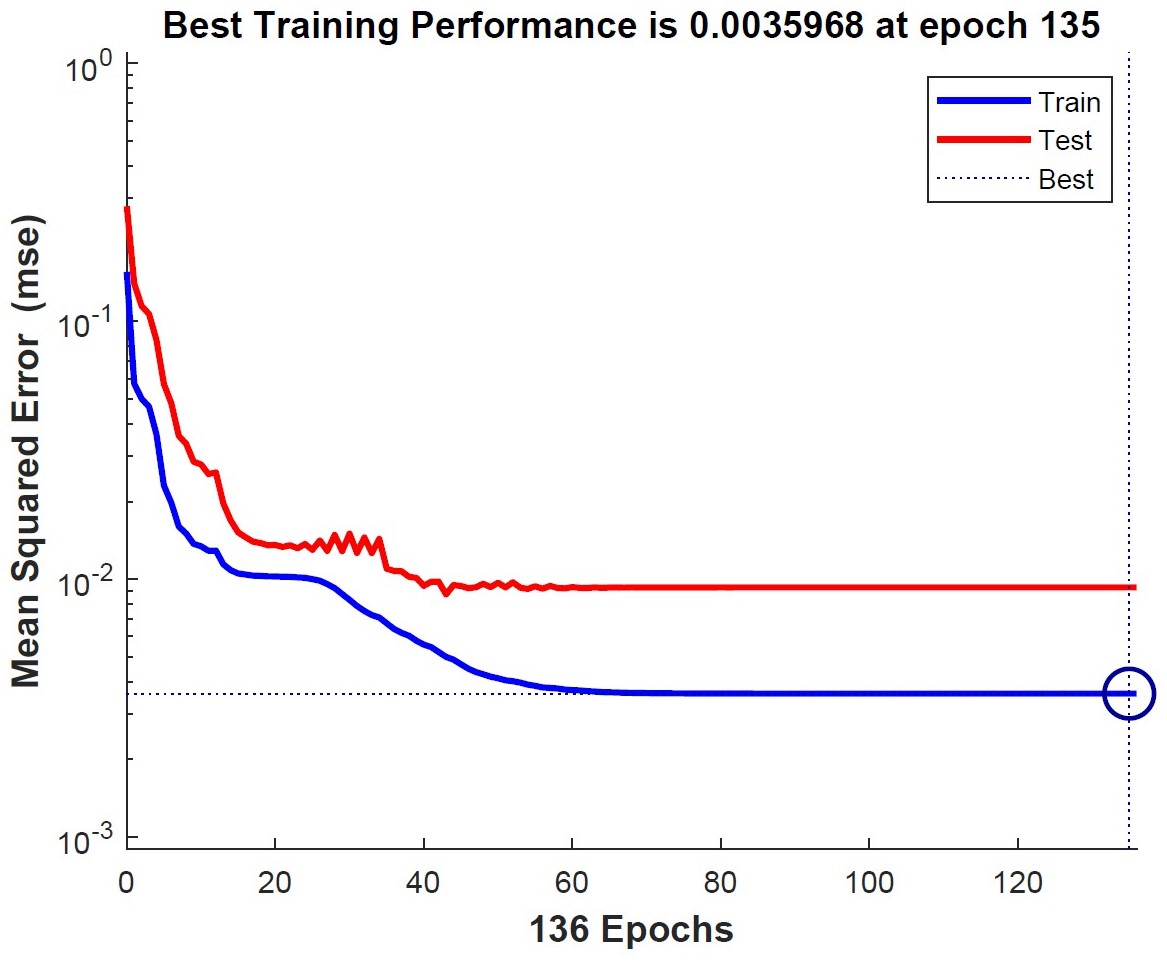
Figure 3: The train set error and the test set error have similar characteristics, which represents a good reliability of our model.
Moreover, the small mean square error of 0.0035968 shows the accuracy of our model.

Regression

Regression model shows how well our model had been trained and how accurate our model predicted. The training accuracy result of our model was shown below through the regression model.

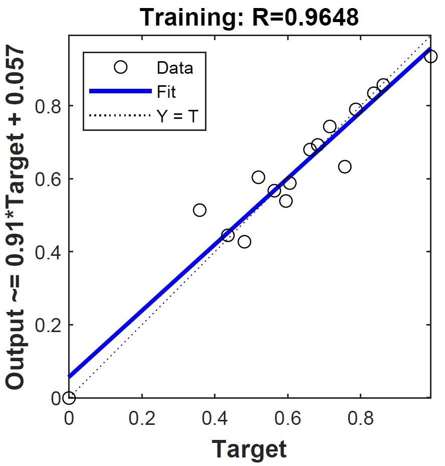
Figure 4: The regression result of training

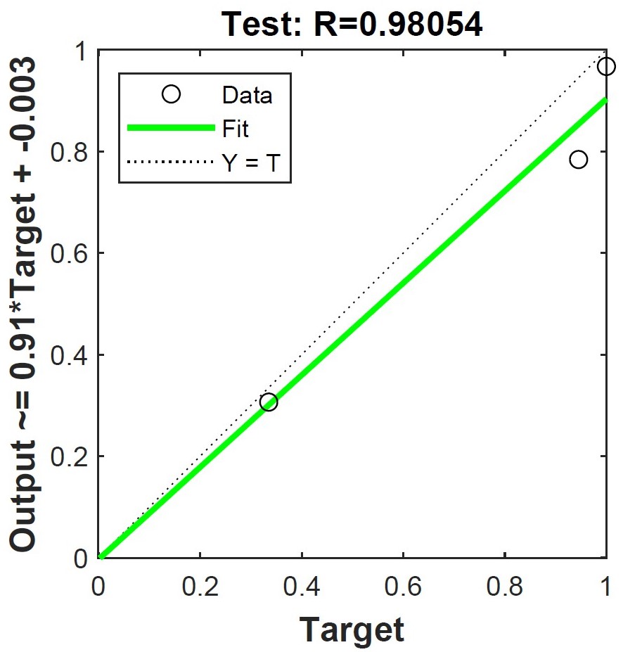
Figure 5: The regression result of test

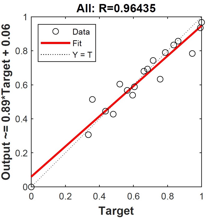
Figure 6: The regression result of total

More Details

All the training results including weights and bias values, parameters, and equations were shown in the code below. If you're really interesting in the detail of our results, please click the button below to see more!

function [Y,Xf,Af] = myNeuralNetworkFunction(X,~,~)
%MYNEURALNETWORKFUNCTION neural network simulation function.
%
% Generated by Neural Network Toolbox function genFunction, 08-Oct-2018 02:58:43.
%
% [Y] = myNeuralNetworkFunction(X,~,~) takes these arguments:
%
%   X = 1xTS cell, 1 inputs over TS timesteps
%   Each X{1,ts} = 3xQ matrix, input #1 at timestep ts.
%
% and returns:
%   Y = 1xTS cell of 1 outputs over TS timesteps.
%   Each Y{1,ts} = 1xQ matrix, output #1 at timestep ts.
%
% where Q is number of samples (or series) and TS is the number of timesteps.

%#ok<*RPMT0>

% ===== NEURAL NETWORK CONSTANTS =====

% Input 1
x1_step1.xoffset = [0;0;0];
x1_step1.gain = [2;2;2];
x1_step1.ymin = -1;

% Layer 1
b1 = [0.23675927677470898214;-0.63098819262182737067;0.24618381408376058261];
IW1_1 = [0.0050654773982650811576 -0.18103144215429012309 -0.37951143126028297203;
         0.65951962684049847407 0.29027817917052955998 -0.5096428679218601987;
         0.36779863987598404584 0.35978048669490930722 1.2466465250108169638];

% Layer 2
b2 = 0.11579284002726117353;
LW2_1 = [0.47667513579074882735 0.80893762887468689815 0.84471206418024180618];

% Output 1
y1_step1.ymin = -1;
y1_step1.gain = 2;
y1_step1.xoffset = 0;

% ===== SIMULATION ========

% Format Input Arguments
isCellX = iscell(X);
if ~isCellX
    X = {X};
end

% Dimensions
TS = size(X,2); % timesteps
if ~isempty(X)
    Q = size(X{1},2); % samples/series
else
    Q = 0;
end

% Allocate Outputs
Y = cell(1,TS);

% Time loop
for ts=1:TS

    % Input 1
    Xp1 = mapminmax_apply(X{1,ts},x1_step1);

    % Layer 1
    a1 = tansig_apply(repmat(b1,1,Q) + IW1_1*Xp1);

    % Layer 2
    a2 = repmat(b2,1,Q) + LW2_1*a1;

    % Output 1
    Y{1,ts} = mapminmax_reverse(a2,y1_step1);
end

% Final Delay States
Xf = cell(1,0);
Af = cell(2,0);

% Format Output Arguments
if ~isCellX
    Y = cell2mat(Y);
end
end

% ===== MODULE FUNCTIONS ========

% Map Minimum and Maximum Input Processing Function
function y = mapminmax_apply(x,settings)
y = bsxfun(@minus,x,settings.xoffset);
y = bsxfun(@times,y,settings.gain);
y = bsxfun(@plus,y,settings.ymin);
end

% Sigmoid Symmetric Transfer Function
function a = tansig_apply(n,~)
a = 2 ./ (1 + exp(-2*n)) - 1;
end

% Map Minimum and Maximum Output Reverse-Processing Function
function x = mapminmax_reverse(y,settings)
x = bsxfun(@minus,y,settings.ymin);
x = bsxfun(@rdivide,x,settings.gain);
x = bsxfun(@plus,x,settings.xoffset);
end

Curcumin Transformation Model

After constructing the tumeric model, we also built up a model which can predict the curcumin containment from tumeric's productivity. Some researches showed high positive correlation between curcumin containment and tumeric mass. Thus, we use the data from the papers to build up the transformation model. Moreover, we use our curcumin sensor to fixed the model with current data from our farm.

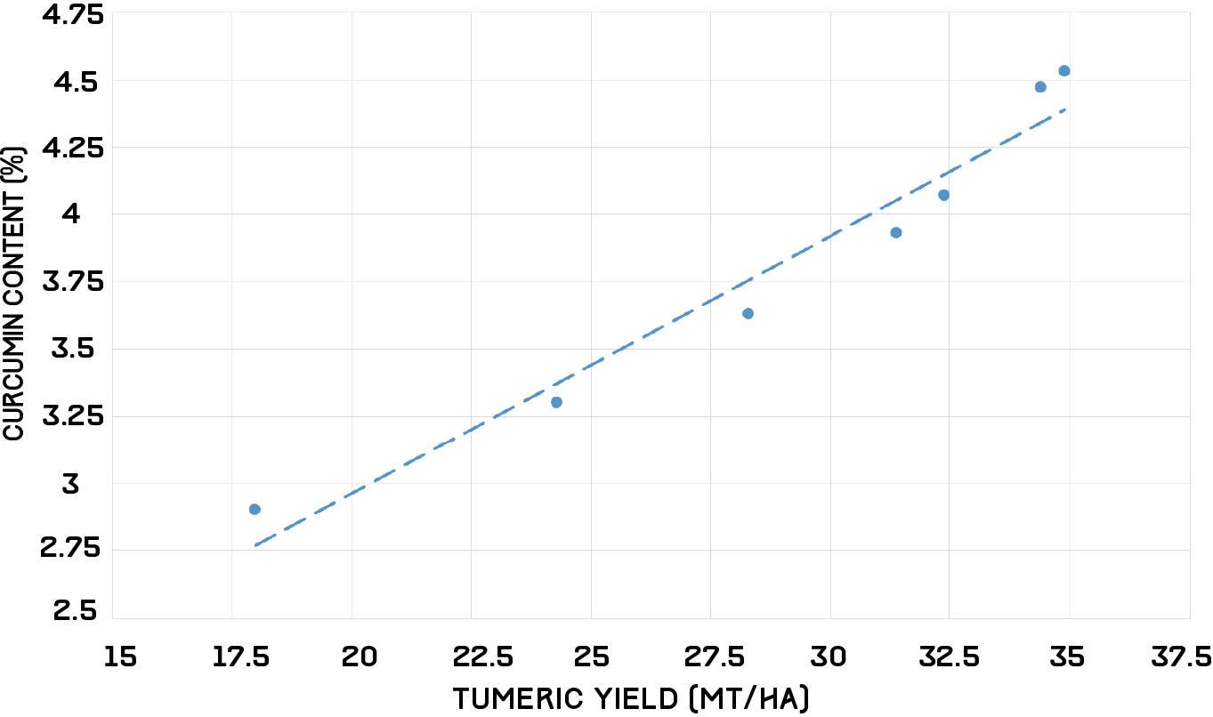
Figure 7: The relation between tumeric yield and curcumin content

According to the data, we got the equation below

$$y=0.0956x+1.0496\qquad where\ R^2=0.9552$$

Productivity from Electrical Conductivity

     Now, we can easily predict the curcumin content through our productivity model. However, currently, there does not exist a real-time sensor that detects nutrient levels in soil. Rather, the two commonly used sensors that detect nutrient levels non-destructively require extraction of soil and analysis in the lab. The first type is an optical sensor that uses reflectance spectroscopy to detect the level of energy in form of reflectance/absorbance by soil particles and nutrient ions. The other type consists of electromagnetic sensors using ion-selective membranes that produce a voltage output in response to ion activity of selected ions, mainly concentrated on H, NO₃, K, Na etc. Both methods are time-intensive processes.

     This year we developed a sensor that can detect levels of the macronutrients nitrogen, phosphorus and potassium by measuring electrical conductivity (EC) alone. This concept stems from a general model we construct relating EC to N, P and K levels through data collected during the process of fertilization.

     From literature^[5] we found that EC to salt concentration can be described by a simple squared function. We therefore began with:

$$ax^2+bx+c$$

We then used our collected data to fit the curve, resulting in:

$$y=-0.0022x^2+0.051x+0.0033\qquad where\ R^2=0.9996$$

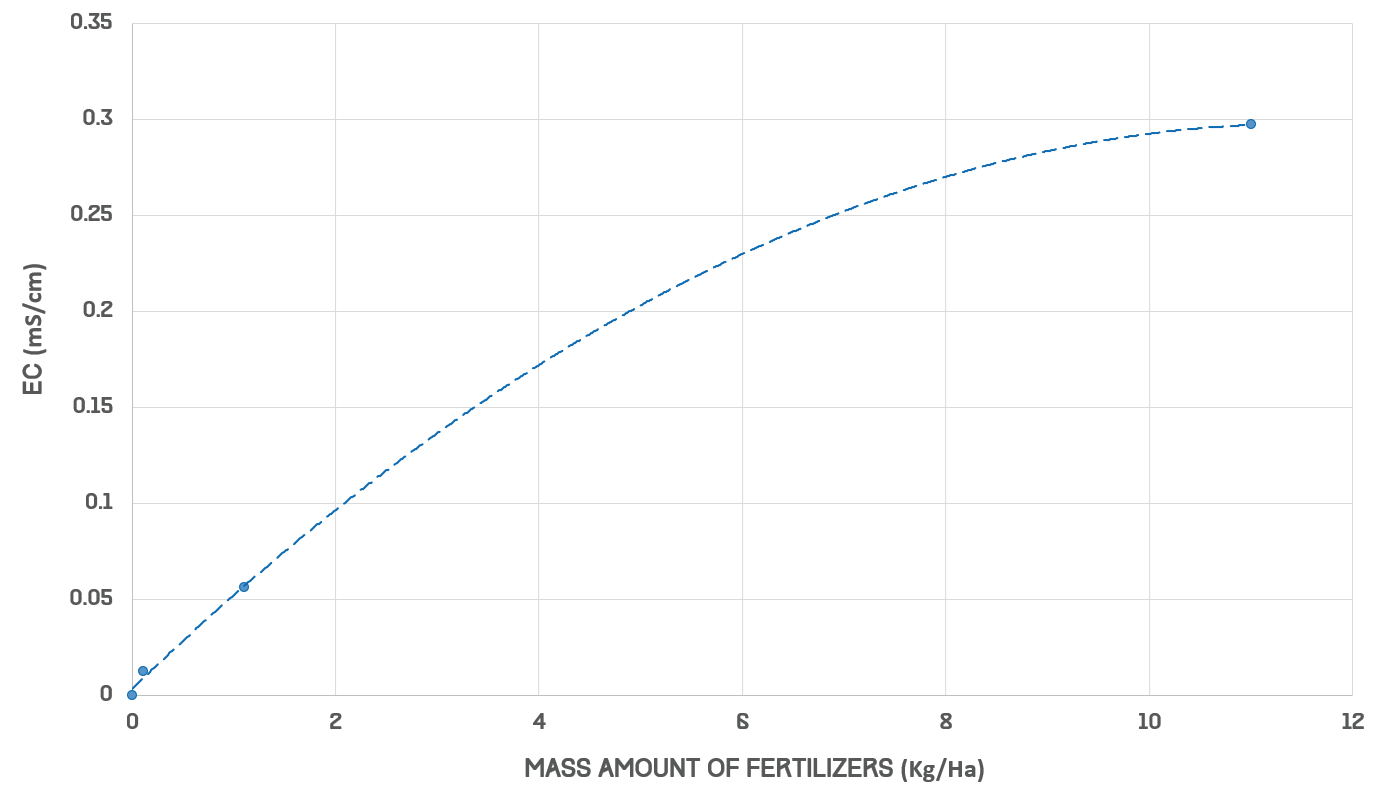
Figure 8: The relation between fertilizer and electrical conductivity

From curve fitting we obtained the following individual equations for nitrogen, phosphorus and potassium:

$$N : 63.253x^2+14.213x+0.180\\ P : 31.626x^2+7.107x+0.180\\ K : 31.626x^2+7.107x+0.180 $$

From these we can directly relate an EC measurement to an amount of fertilizer as long as it is fixed in ratio of N, P, and K. Because we have an EC to productivity model, we can convert our EC reading into an N, P, and K value; comparison with our curcumin sensor allows us to compare our actual curcumin concentration with predicted value, strengthening our model.

Conclusion

Through the concept, we built up the world's first productivity model which can accurately predict the productivity with barely nutrients amount in the soil. In the future, our productivity model can be applied to any crop the farmers want simply by training the model with validate data of the crops.

If you are interesting in our model, please click the icon to find out how them work in GitHub!

References

1. Akbar, A., et al. (2016). "Development of Prediction Model and Experimental Validation in Predicting the Curcumin Content of Turmeric (Curcuma longa L.)." 7(1507).
2. Negnevitsky, M. (2005). Artificial intelligence: a guide to intelligent systems, Pearson Education.
3. Ramana Reddy, D. V., et al. (2015). "Soil-Plant-Fertilizer Relationships in Turmeric Assessment of Soil-Plant-Fertilizer-Nutrient Relationships for Sustainable Productivity of Turmeric under Alfisols and Inceptisols in Southern India." Communications in Soil Science and Plant Analysis 46(6): 781-799.
4. Sumathi, C., et al. (2010). "Influence of biotic and abiotic features on Curcuma longa L. plantation under tropical condition."
5. Brinkmann, T., et al. (2002). "Non-linear calibration functions in ion chromatography with suppressed conductivity detection using hydroxide eluents." 957(2): 99-109.