Team:Calgary/Model
MODELLING
Introduction
The goal of the modelling was to assess inlet positioning on our reservoir design, and to reduce the difference in fluid path resistance. Decreasing the differences in path resistance assure uniformity of fluid flow at any of the outlets, which is advantageous in our system. Previous work has shown that inconsistent flow rate in flow-focusing microfluidics causes backflow in different streams, and disturbs the system's ability to produce uniform droplets. To model our system, we used the COMSOL Multiphysics software.
Our Modelling Process
Using COMSOL, we set up the geometry in which the fluid is filling and the outlets are on the bottom of the reservoir that correspond to the inlets on the glass chip. After setting up the geometry for fluid path, we set the model to solve for a time-dependent state; up to right before the reservoir reaches a steady state. This was done in order to see if any of the initial conditions were causing an unexpected error, which would affect our final results. The time dependent solver for incompressible fluid flow is defined by the Naiver-Stokes and mass continuity equations.

Figure 1. Top: The Naiver-Stokes equation describes motion of viscous fluids. Bottom: The continuum equation describes the conservation of mass
Here, ρ is defined by fluid density, δu/δt is the first order partial
derivative of velocity with respect to time, u is the fluid velocity, ∇ is the divergence
operator, P is pressure, μ is fluid viscosity, T is the transpose operator, l is path length,
and F is the gravitational force on the fluid.
We defined the geometry outlets using the "physics: outlet" feature, the
inlet position that we were testing from "physics: inlet", and the rest of the geometry was defined
to be in contact with a wall.
Three large assumptions were made to describe this model. First, it is assumed that flow in the device will be contained in the laminar regime. Laminar flow is when a fluid flows without any disruption between streamline layers. We assumed this because fluid velocities exiting the reservoir are extremely low, and the path does not contain any bends, which is favorable for the laminar regime.
The second assumption is that the fluid inside the reservoir is incompressible. We assumed this because at no point in the model, or in the physical application, should there be pressure that are high enough to compress fluid. Also since we will be working only with liquids, which are generally assumed to be incompressible in most applications, we should set the model to solve for non-compressible fluids.
The third assumption is that there are no parts of the model operating in microfluidic flow regimes. This is because this model has been developed to optimize the pressure differential leaving the reservoir. So, inertial forces due to gravity are present. Indirectly, this also leads to defining motion at any wall as "no-slip". The no-slip condition is the behavior that a fluid moving through a medium will have a velocity of zero at the interface between fluid and medium. Some microfluidic systems have shown that they do not obey the no-slip condition, but this is dependent on the system in consideration. Since the reservoir seems to be large enough, we have assumed that the no-slip condition is applicable to our model.
We were interested in getting two sets of data from our model. They
are the velocity as a function of radial position, and the pressure as a function of radial
position. We were interested in obtaining these values as the system is approaching steady state,
to assess what the pressure differential as during continous flow. This is why the results are
the solution of the last time step. Solving for this can be defined in COMSOL.
Results
An initial observation from the 3D velocity-slice model illustrates the gradients that were expected at the inlet and outlets. We based our model to flow at 20 microliters/minute; This value has been reported to work in microfluidic droplet generators with similar flow-focusing geometry.
Figure 2. 3D Velocity-slice diagram of reservoir filling
To assess the velocity values at the outlets of the reservoir, we redefine the fluid velocity as a function of radial position. This is done using a plane-cut and line-cut command native to COMSOL. From here on, the results are discussed in reference to the outlet labels shown in figure 2.
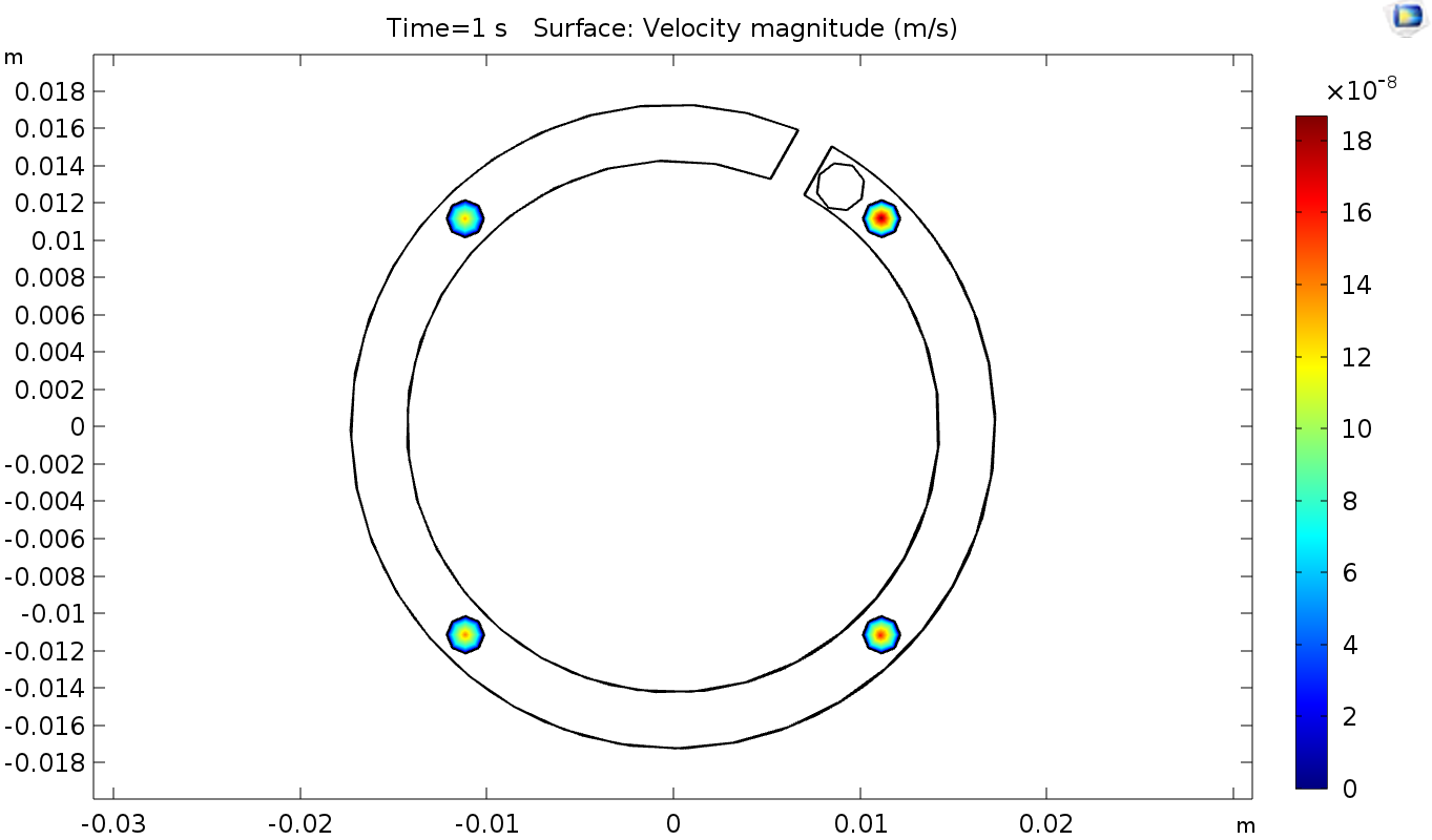
Figure 3. 2D projection of reservoir, illustrating velocity magnitude of outlets
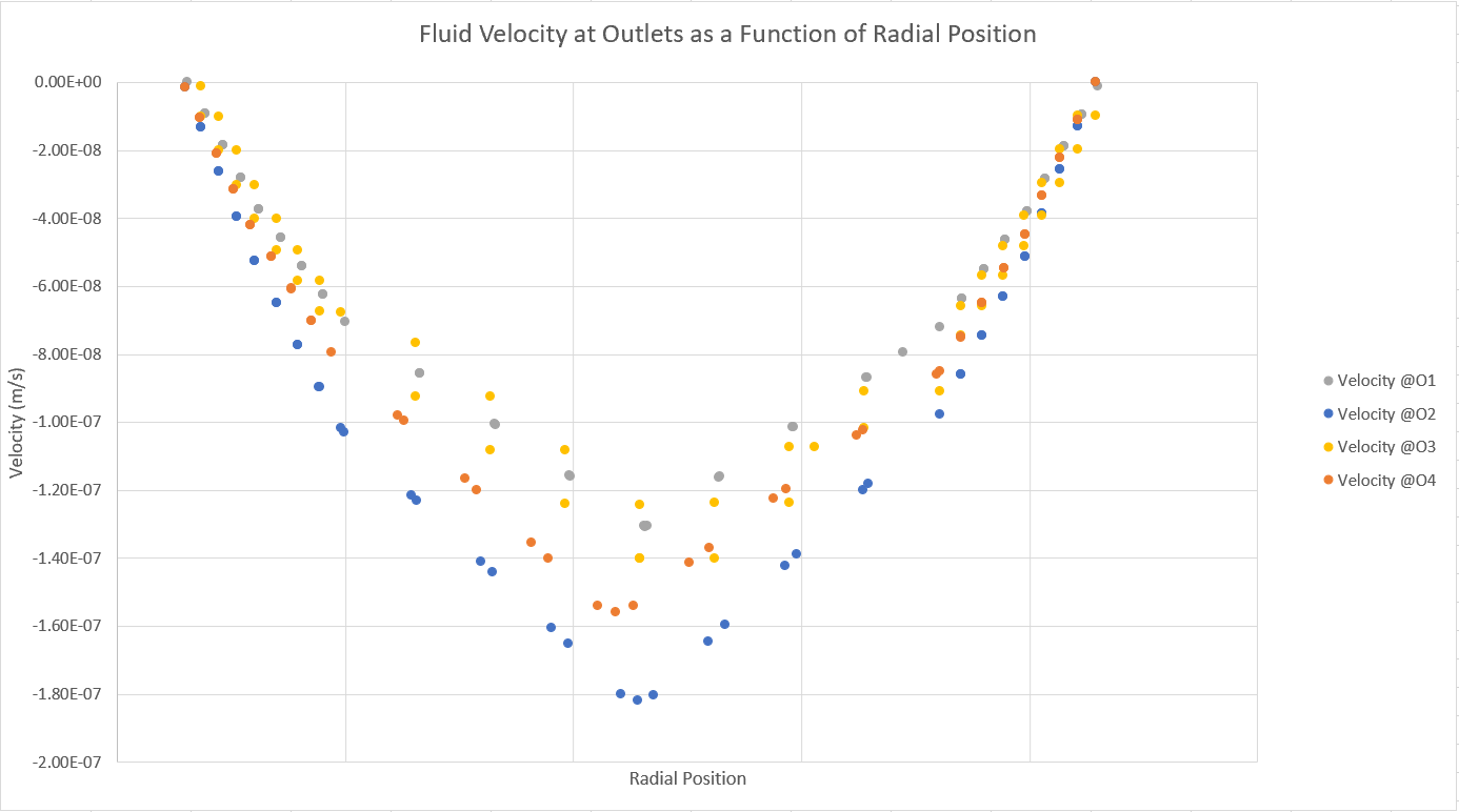
Figure 4. Fluid velocity at outlets as a function of radial position
Our model performed velocity calculations on 47 different radial points for each outlet. From Figures 2 and 3, it can be seen that O2 has the greatest velocity magnitude and the largest maximum velocity value. This can be explained by the proximity of the fluid inlet (I1) to O2. This is further shown as the maximum velocity of O1, which is -1.31*10-7m/s is the lowest maximum value of the other outlets, while it is also the farthest.
Like before, pressure values were calculated at 47 different radial points at each outlet. However, figure 4 illustrates the difference in pressure drop near the center of the outlet seems to be smaller than those of the velocity value. This can be seen in the 3D pressure contour in figure 5, as the lines around O2 and O4 correspond to pressures in the range of (52.46 to 42.65)*10-7Pa, while O1 and O3 correspond to (42.65 to 37.75)*10-7Pa.
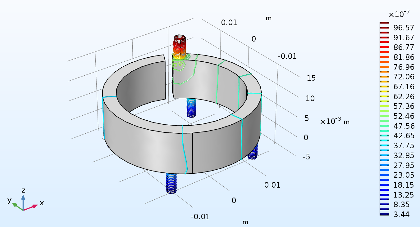
Figure 5. 3D Pressure contours of reservoir at the last time step
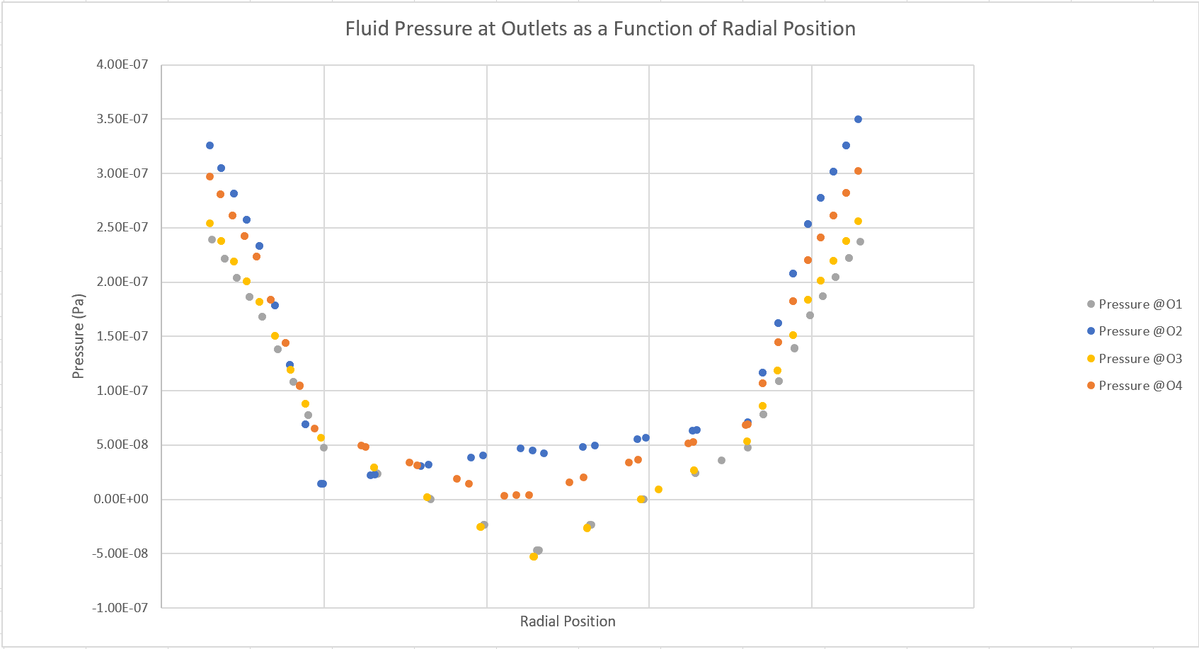
Figure 6. Fluid Pressure at Outlets as a Function of Radial Position
This result emphasizes the importance symmetric position for the inlet with respect to the outlets. To confirm the results of the model, we built the reservoir as designed. However, moving forward we will iterate on the position of the inlet, and compare the results to determine which position will yield convergent velocity results.
WORKS CITED
Colin, S. (2010). Microfluidics. London: ISTE.
Headen, D.M., Garcia, J.R., Garcia, A.J. (2018). CPArallel droplet microfluidics for high throughput cell encapsulation and synthetic microgel generation. Microsystems and Nanoengineering, 4, 17076. doi: 10.1038/micronano.2017.76.
Li, W., Young, E., Seo, M., Nie, Z., Garstecki, P., Simmons, C., Kumacheva. (2008). Simultaneous generation of droplet with different dimensions in parallel integrated microfluidic droplet generators. 4, 258-262. doi: 10.1039/b712917c
Young, D.F. (2011). A brief introduction to fluid mechanics (5th ed.), Hoboken, NJ: Wiley.