Team:Grenoble-Alpes/Model
Template loop detected: Template:Grenoble-Alpes
MODELING
In order to optimize the lysis step in our system, we used a modeling of the interaction between phages and bacteria. However, the purpose of this system is also to promote therapy. With this in mind, we used our modeling to give the doctor a tool to optimize the therapy dose needed by the patient.
After working on this model for some time we reached out to Ruth Bentley from the Nottingham iGEM team, we were able to work together and to discuss different modeling aspects.
It is important to note, that even though we worked on a lot of the theory together, we implemented the model with different languages, as Ruth coded on python and our work was done in Matlab.
All our modeling codes can be found here
DownloadFor our modelling we based ourselves on an article [1], in which the authors model the interactions between phages and bacteria using the following equations:

Where:
S is the number of susceptible bacteria (the one that can be infected by phages)
R is the number of mutated bacteria (the one who became resistant to phages)
I is the number of infected bacteria, and therefore will be killed by the phage after a latent time
V is the number of phages
The parameters are described in the table below:
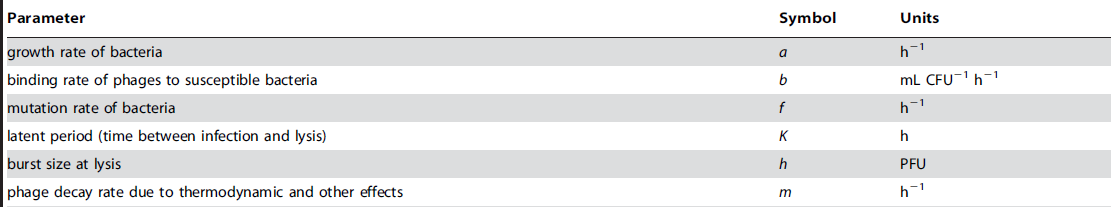
We can represent the situation with the following graph:

Let’s explain each equation :

The variation of the number of susceptible bacteria S over time is:
A gain equal the growth of those bacteria: +a*S
A loss equal to the number of bacteria that mutates into phage-resistant bacteria: -f*S
A loss equal to the number of bacteria infected by phages: -b*S*V

The variation of the number of resistant bacteria R over time is:
A gain equal to the growth of those bacteria: +a*R
A gain equal to the number of bacteria that mutates into phage-resistant bacteria: +f*S

The variation of the number of infected bacteria I over time is:
A gain equal to the number of bacteria infected by phages: +b*S*V
A loss equal to the number of bacteria infected by phages at time t-K (where K is the time needed for a phage to kill a bacterium): -b*S(t-K)*V(t-K)

The variation of the number of phages V over time is:
A gain equal to the number of phages released after the lysis of previously infected bacteria, where h is the average number of phages created inside an infected host: +h*b*S(t-K)*V(t-K)
A loss equal to the number of phages that infected bacteria: -b*S*V
A loss equal to the degradation of phages in the solution: -m*V
As we can see the equations here are relatively simple, and the only real difficulty to solve them is the presence of a Delay Differential Equation (DDE) in the form of S(t-K)*V(t-K).
To solve those equations we chose to use MATLAB because we were used to this computing language (and because we obtained a license through the iGEM competition framework). Thanks to this computing environment we can solve those DDE with a built-in function called “dde23”.
This function comes with some options, one of which allows us to indicate the function what happens for t < K. In our case, we want that for t We started by implementing the system as described in the article, then to obtain equations that fitted our need we added :
A variable D representing the quantity of DNA freed during the lysis of the bacteria by the phage A carrying capacity C (modeling the fact that a solution can be saturated in term of bacteria) A degradation factor r (for bacteria) and l (for DNA) A factor d modeling the average quantity of DNA freed after lysis Here are the final equation in our code: It is important to note that we were able to implement the DNA variable D quite easily because we did implement a toxin variable in order to work with Ruth from the Nottingham iGEM team. After working with Ruth we also decided to use a carrying capacity factor. And we ended up agreeing on the fact that the carrying capacity is a common factor for both S and I (therefore (S+R+I)/C and not (S+I+R3)*C. Thanks to our iGEM Meet’up in Marseille we were able to explain the first version of this modeling and on the advice of one of the participants we looked into implementing a tool for comparing the different type of phages-bacteria interaction. We would have like to do this with as many phages as possible, unfortunately we did not manage to obtain key parameters for a lot of different strains of phages, therefore we only offer to the user the possibility to choose between 2 phages-bacteria interaction: C.jejuni and C.difficile for which we had complete set of parameters (respectively thanks to this article and to our partnership with Nottingham). However, we offer to the user to choose an interesting set of parameters, that are not related to any particular strain of phage, but show the wide spectrum of different interaction possible. We also added the possibility for the user to change any parameters after he chose one strain of phage. We implemented 5 interesting set of parameters: High phages multiplication Fast-growing bacteria Low phages binding rate Slow lysis Low carrying capacity In order to give a more user-friendly modeling to the user, we implemented 3 interactive dialog prompt. The first one allows the user to choose the phages-bacteria interaction: The second one allows the user to choose the initial population of phages and bacteria. It also allows the user to choose 2 parameters that have an impact on the computing time: timespan and accuracy of the modeling. And finally, it gives the user the option of choosing a file name for the modeling figure that will be saved as an image in the current folder at the end of the process. The third one allows the user to change directly the key parameters of the system modeling. Here is an extended view of the following graphs' legend. If there are no phages added to our solution, the bacteria grow normally until they reach the carrying capacity (number of bacteria at which the solution is saturated) of the solution, which is an equilibrium state for our system. If there are no bacteria, the phages slowly degrade. This figure shows the result of our simulation for a phages-bacteria interaction that do not present any extreme value for the key parameters. When we change the growing rate of our bacteria it is interesting to see that the time necessary to eradicate the bacteria is actually smaller than in the average behaviour modelling. This can be explained by the fact that when the growing rate is higher the bacteria population is close to the carrying capacity for a longer time. With a higher phages multiplication rate even less time is needed to eradicate the bacteria population.
We can also see here two “bumps” in the number of phages and DNA released, they occur after one and two TL (latent time). Those bumps can be seen because of the very high number of phages released after lysis, called the burst size and set here to 500 instead of 20 for the average behaviour.
In this case we switched the latent time TL from 36 minutes to 10 hours (compared to the average behaviour). We can here see that the number of phages takes more time to achieve the tipping point where the bacteria population start declining. In the case of a low phages binding rate Ki there is a slower decline of bacteria, or even an equilibrium state with both phages and bacteria as it is the case in this situation. Interestingly an equilibrium state can also occur when the carrying capacity is too low. This situation is explained by the fact that the number of infected cells I is equal to the product of the binding rate Ki, the number of phages V and the number of susceptible bacteria S. Therefore if the number of bacteria S is capped by the carrying capacity, the number of phages and infected cell is also limited.
This figure shows the result of a phages-bacteria interaction where the phage is not effective at killing the bacteria. This case was inspired by the work of Nottingham 2018 iGEM Team, who worked with lysogenic phages. Lysogenic phages end up by multiplying and killing their host, but not in every case, and with a long latent time. Finally we also kept the implementation of the resistant bacteria in our model based on this article[1]. We can see here a case with a strong resistance factor. The number of susceptible bacteria (the one that can be infected by phages) quickly decrease as we have seen before. This allow the phages-resistant bacteria to grow. Finally Ruth gave us the idea of computing this 3D figure: The idea behind this figure is that the doctor wants to know how much phages he has to administer in order to obtain a certain amount of bacteria after a giving time.
From this graph we can actually see pretty easily than the most important factor is the time and not the targeted bacteria population that has to be reached at the targeted time. [1] Cairns BJ, Timms AR, Jansen VAA, Connerton IF, Payne RJH (2009) Quantitative Models of In Vitro Bacteriophage–Host Dynamics and Their Application to Phage Therapy. PLoS Pathog 5(1): e1000253. doi:10.1371/journal.ppat.1000253

Implementing a tool to compare different type of phages-bacteria interaction:
User interface:


Results:

1) No phages

2) No bacteria

3) Average behaviour

As we can see after a small time where the phages population is steady it quickly rises. This small time is the result of the time needed by the phage to multiply and kill its host after infection. This time is called the latent time TL.
Once there are enough phages the bacteria population start to decline due to the multiple phages-induced lytic cycles. In this modeling (with no phage-resistant bacteria factor) we can see that there are no more bacteria after 23 hours.
As soon as bacteria are killed their DNA is released into the solution, this DNA will then be degraded over time.
Finally, we can see here that the bacteria population is equal to the carrying capacity (and the number of bacteria in a “no phages” situation) for a certain amount of time, then starts to decline.
This “typing point” is in fact reached when the phages-bacteria ratio is high enough.
In this article[1] the authors already highlighted this threshold: “the concentration of susceptible bacteria can only decline if the concentration of free phages exceeds the inundation threshold VI”. In our modelling with our equations this threshold is equal to:

4) Fast growing bacteria
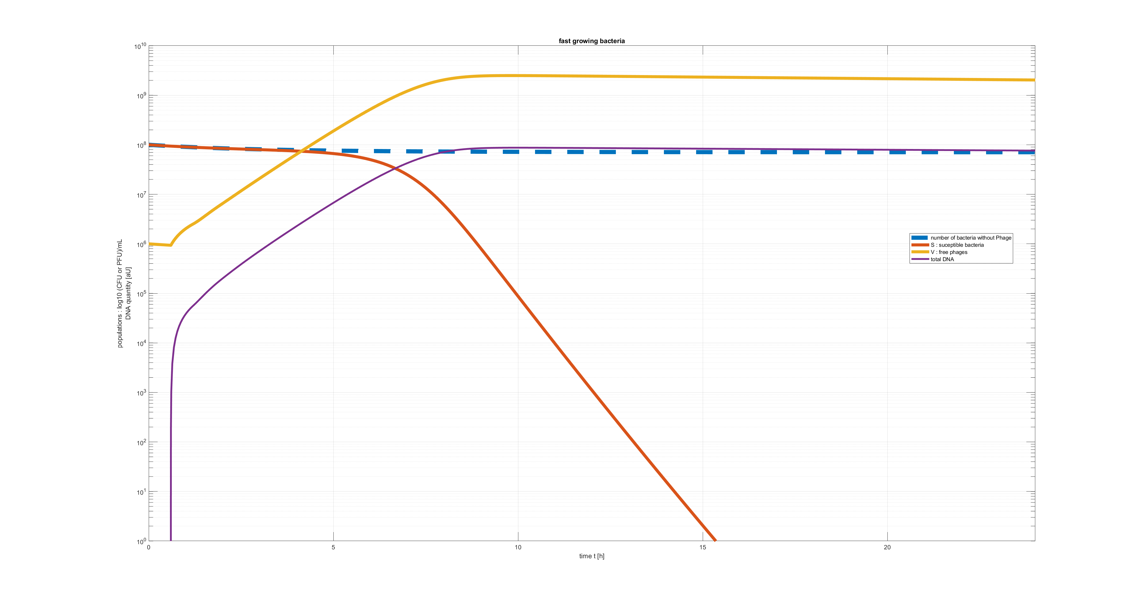
As a result there are more phages-bacteria interactions and more phages produced, which in the end eradicate the bacteria more rapidly.
5) High phages multiplication rate

6) Slow lysis

The bumps linked to the release of phages after TL and described in the previous case are also very easy to see here.
7) Low phages binding

This shows the importance of the binding rate for a phage therapy.
8) Low carrying capacity

9) C. difficile

We implemented this situation in our MATLAB modeling by changing the lysis time, but also by adding a lysis probability factor pL: only in a few percentage of the case will the infection end up in a lytic cycle.
As we can see the phages-bacteria interaction has a cyclic behavior: once the phage reduced the number of bacteria there is an equilibrium phase, but the phages population start to decline due to the phage degradation factor, allowing the bacteria population to rise again.
The rise of the bacteria is not quickly controlled by the phage due to the long latent time. But after a while, the number of phages reaches again the inundation threshold VI and the bacteria population starts to decline again.
10) C. jejuni

However the decrease of the susceptible bacteria population could be enough for a phages therapy: once the total number of bacteria is low enough the immune system of our patient will take over from here and kill the remaining bacteria.
Phages needed for a therapy:

REFERENCES