Modeling

Modeling proved to be an invaluable tool during both the design and testing phases of our CUTSCENE project. In order to construct this complex recording circuit, we needed to understand not only steady state outcomes, but the dynamics of the system as well.

We tackled this challenge by breaking down our key goal (i.e. does CUTSCENE work as intended?) into smaller questions, focusing on both storage and retrieval of our signal of interest. As a direct result, our group was able to update the design of the system and gain insight into a variety of performance testing methods.

Acheivements

Built an accurate model of the base editing system using a variety of recursive bayesian estimation techniques, including extended kalman filter and particle filter methods

Used initial readout predictions to improve the design of our system and induce a more digital behavior

Extended 2017 British Columbia’s cas9 off-target modeling by expanding the scope to include base-editing mistakes

Developed a software tool to convert sanger sequencing readouts (read more about CrisPy!) into stimulus data

Figure 1: Cutscene workflow can be categorized into two stages: recording and playback

Questions about Recording

Can we accurately model the recording circuit?

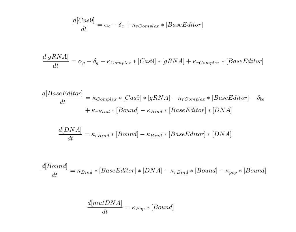
Because the cas9 base editor lies at the heart of our recording system, it was essential that we understood it's dynamics and regulators clearly. The first step we took in designing a model for this component was specifying all major elements and relationships. The binding kinetics for cas9 and DNA are not fully known, but have generally been broken down into the following stages: PAM recognition, DNA melting, R-loop formation, DNA cleavage/mutation, and dissociation DNA dissociation [Salis, Raper, Mekler]. To simplify our interactions, we chose to combine the first three into a single binding step. The point mutation and subsequent dissociation are also combined into a single step, since it is known that unbinding is rate limiting. We choose not to use the Michaelis-Menton type equations for enzymatic reaction since it assumes that substrate exists in much larger quantities than enzyme. In this scenario, we also assume that both the promoter for cas9-base editor and its associated gRNA are turned on, leading to a constant production rate.

After having listed out our reactions, we then defined our differential equations using mass action-kinetics:

Figure 3: Base editing differential equations

How do we find appropriate kinetic parameters?

One of the key challenges to any rule-based, biological model is finding a functional set of kinetic parameters. Often it is difficult or impossible to directly measure the rate constants for every single step, and so these values are instead obtained by fitting the model to experimental output.

Still, we began our search by pouring through the literature for previous kinetic estimates. The full table of values is shown below:

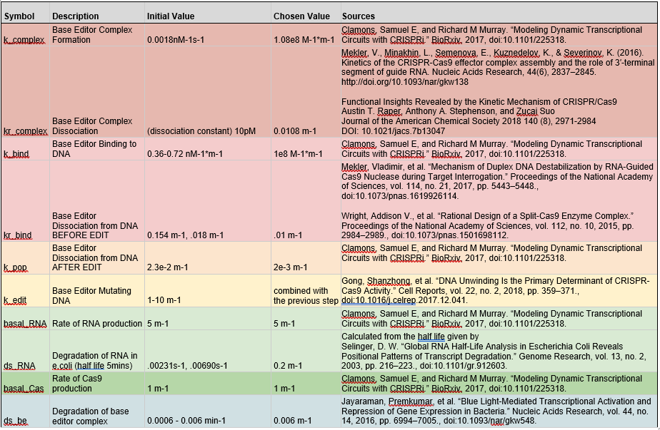
Figure 4: Literature values for each kinetic constant

One of the biggest issues that we noticed with these estimations was that they were made for normal cas9 and not our specific base editor. Additionally, many experiments were conducted outside of bacteria, instead using only the isolated molecules of interest. We suspected that consequently many of these estimates were too fast, which was supported by initial model runs producing much higher base editing rates than experimental data had suggested.

Previously, teams have used regression and maximum likelihood estimation (MLE) methods to converge on their parameters of interest. However, these techniques fail to fully take into account process and measurement noise, resulting in issues when trying to fit sparse and error-prone biological data [Lillaci, X. Liu]. Markov chain monte carlo (MCMC) methods fair better, but still are limited computationally, as they must generate a full numerical ODE simulation for each step they make through their parameter-space.

By using recursive bayesian filters, we were able to quickly update our estimates with each new measurement, despite using relatively few and noisy data points. This technique provides other notable benefits as well. In particular, the filter allows for A) the fusion of multiple measurement types B) testing for assumptions about the model itself.

Recursive Bayesian Filters

Recursive Bayesian filters (also known as Sequential Bayesian filters when applied to time series data), have been heavily studied for applications in robotics and control systems. More recently, researchers such as Lilacci and Khammash have transferred the techniques to the biological domain [Lilacci et al].

Both versions (Extendend Kalman and Particle Filters) of the recursive bayesian estimator work by treating the biological system as a hidden markov model, in which the next state of the system (in this case a vector of all element concentrations) is only dependent on the previous state. It is assumed that an outside observer cannot measure these states directly, and therefore must rely on indirect measurements that are a produced by a separate output function. Stochastic variation can occur either during the state transition (process noise), or during measurement (measurement noise).

Figure 5: A standard depiction of the hidden markov model

Estimation Steps:

A good general example for how the sequential bayesian filter functions is the kalman filter, which is commonly used to track simple linear systems. It consists of a two main steps: prediction and update. In the predict step, the system plugs the previous state and covariance estimate into a user-defined function and finds a new state and covariance estimate, called the a priori distribution. Then in the update step, this calculated state and the new measured state (likelihood distribution) are combined together through a weighted average to form the posterior distribution. The weights correspond to the covariances of each state, so that a measurement with a wide distribution (high variance) is trusted less than one with a very narrow distribution (low variance)

Figure 6: Depiction of the a priori, likelihood, and posterior distributions [*Artificial Intelligence for Robotics*, Georgia Tech, 2018]

State Extension:

In order to modify this prediction system for use with parameters, we need to use the idea of state extension. This means treating each of our parameters as an additional state variable, whose predicted change each time step is 0. Just as the filter will converge on the most likely position of a robot, so too will it tend to converge on the most likely parameters that fit the model.

Extended Kalman Filter:

Our first attempt at parameter estimation used an Extended Kalman Filter (EKF). Unlike the normal Kalman filter, this filter is able to predict nonlinear dynamics. Therefore, instead of directly using our prediction function to update the distribution, we first had to linearize it. This process is similar to taking the tangent of a curve at a certain point, but in a higher dimensional space. Using the jacobian matrix of our reaction equations, we were able to construct a filter that could track moderately non-linear systems.

Despite its popularity, the Kalman filter does have its drawbacks. Firstly, it assumes a normal distribution, which may not always be the case in biological systems. Secondly, unlike the linear kalman filter, an Extended Kalman filter is not mathematically guaranteed to converge on correct estimates, especially when tracking highly non-linear systems. An intuitive way to reason why this error occurs is to think of a line tangent to a function of very high curvature. Even after small deviations from the intersection point, the tangent line diverges sharply from the function. This error translates to deformed distributions in the case of the extended Kalman filter.

Particle Filter:

After discussion with Dr. Ahmed Dallal of the University of Pittsburgh’s ECE department, our team decided to also explore another type of sequential bayesian filter called a particle filter. Just like the kalman filter, this method has a predict and update step, but instead of using covariances to track the shape of the distribution, this method uses a number of points scattered throughout the state space. Each of these points transition to the next time step based on the prediction function, forming the a priori distribution. Next the update process happens in two parts: Each particle is assigned a weight corresponding to its distance from the measurement, and then this weighted distribution is sampled to form a new posterior distribution. There exist a variety of resampling methods available, but we chose to use systematic resampling in accordance with results from Hol, Schon, and Gustafsson [Hol et. al]. This helps the filter to converge faster and to prevent sample degeneracy, in which particles collapse to a single state and fail to represent the correct distribution.

While more demanding computationally, the particle filter is able to consistently track arbitrary distributions with non-linear dynamics. Simulations using thousands of particles could still be conducted on the scale of a minute using a standard laptop.

Example of 1000 particles going through the predict/update cycle

Filter Testing:

To ensure that our parameter estimation methods could produce unique and identifiable results, we put them through two tests. First, we first tested them on a toy example in which parameters were known. Afterwards we moved on to the more complex set of equations believed to be governing the base editor reactions, but simulating data with literature values of parameters.

In the toy example, we established the equations for a simple binding model, where two components A and B combine to form C. We chose 1 min-1*M-1 for the forward rate constant and 0.1 for the reverse, and then simulated the results using a stiff ode solver (matlab ode15s). We then added artificial measurement noise (gaussian, variance of 1 nM at about 10% of the total range).

Figure 7: Simulated concentrations of product and reactant in the toy example. Measurement noise is added to mimic experimental data

To better simulate actual conditions in which literature values could be wrong, initial parameter estimates were each an order of magnitude lower than their actual values (0.1 and 0.01). We also used as few data points as possible while still maintaining small error rates (<10%). For the extended kalman filter, the lower limit turned out to be 30-40 measurements, while the particle filter had success down to 15.

EKF Test #1:

Figure 8: EKF simulation run on the toy example. Reactant and Product tracking is shown in the top two plots, while the two parameter estimates are depicted in the lower two.

As recommended by Lilacci and Khammash, final parameter estimates were calculated by averaging the last ten kalman filter predictions. Running the entire simulation 1000 times resulted in a mean parameter estimate of 0.9951 and 0.0968 respectively (less than 1% and 4% error), with standard deviations at about 10% each. As seen in the figure above, two different measurement types (reactant and product concentration) can be fused together to produce more accurate results.

Figure 9: Distribution of parameter estimates over the course of 1000 EKF simulations

EKF Test #2:

Next, we moved on to testing our filters with the predicted equations of our base editor system. We chose to focus on the base editor binding to DNA and . We again simulated the data using known constants (taken from the literature), and measurement noise with variance around 10% of the total range. Unfortunately, because our system was very non-linear (due to the wide range of rate constants), the extended kalman filter diverged from the correct estimates. It was clear that a different filter would be needed for this more complex system.

Particle Filter Test #2:

The particle filter was initialized with 1000 particles and fed the same simulated data as the EKF. This time the filter was able to eventually track the amount of DNA base edits over time, and converge onto the given parameters. As shown in the figures below a tradeoff still existed between the number of datapoints used and the accuracy of results. The 10% error threshold was crossed between 30 data points and 15 data points, but estimates could still be improved by altering the time steps between points, giving more resolution to the transient stages of the reaction.

Particle Filter Results:

Once the particle filter had been shown to correctly converge on given parameters, it was time to test with information from actual experiments. Data on mutation frequency over time was taken the David Lu lab’s CAMERA paper. The 8 time points were interpolated using a spline fit to get a total of 16 steps. This was then fed into the particle filter using 100,000 particles (~5 min runtime). One important improvement that was made at this stage was calling the predict function at time intervals between experimental data points, in order to reduce the error of our numerical ODE solver. Simulation results are shown below:

Figure 10: Particle Filter simulation run with 100,000 particles. DNA mutation frequency is shown in the top plot. And K-bind, K-rbind, and K-pop values are depicted in the subsequent three.

Even with initial parameter guesses an order of magnitude different (shown in blue), the particle filter quickly converges on new parameter estimates within a few data points. Tracking of the DNA mutation frequency (shown in the top plot) is illustrated in the top plot, with experimental data shown as blue points and particle filter estimates shown in black. Taking an average of the last 10 estimates, K-bind was calculated to be 0.0041 M-1*min-1, k-rbind was calculated to be 0.051 min-1, and k-pop was found to be 2.3102e-4 min-1.

Figure 11: Comparison between experimental data and model with updated parameter estimates.

Will the system produce an identifiable readout?

Once the base-editor equations and their associated parameters were defined, we could then move on to predicting the behavior of our recording plasmid. Ideally, we hoped that the base editor would shift our “reading frame” in a predictable fashion. The figure below depicts this idealized behavior in the form of logic gates. In the optimal scenario we would induce the production of base editor, which would make mutations to our DNA at a constant rate (symbolized by delay elements). Consequently, this editing would allow the next DNA frame to be written to (symbolized with AND gates) after a set period of time. However, we suspected from the beginning that we would observe something much less digital in our biological circuit.

Figure 12: Logic diagram for recording circuit

To address this timing concern, we incorporated our base editor equations into a larger model. Instead of just mutating one piece of DNA, we assumed that the first mutation would open up the next DNA frame to be modified, that the second mutation would open up the next, and so on. By pretending that the DNA was essentially transformed into another species, we could then track the strength of each reading frame over time. While not entirely predicative of the final readout (the decay time of the stimulus gRNA plays a large role in exactly how many mutations get written where), if the frame shift timing was extremely nonlinear and messy, then the final readout would almost certainly be as well.

We made use of the BioNetGen ode simulation method (which in turn makes use of the cvode library of ODE solvers) and suite of visualization tools to generate our estimations. Our initial circuit design was simulated over the course of 20,000 minutes (~14 days), with results pictured below:

Figure 13: Bionetgen simulation run with a single gRNA. Targets can be written to as soon as the previous one has been mutated. Comparison to CAMERA experiment shown in the top right.

Comparing to a similar experiment conducted in the DOMINO paper, these predictions seem to be accurate. While in some cases it would be plausible to use these predictions as way to classify our readouts (for example A% of target 1, B% of target 2 corresponds to time point T), we worried that the signal to noise ratio would be too small to distinguish timepoints across a large section of the recording window.

In order to more clearly differentiate between timepoints, we needed a way to convert our signal into something more digital. One way to do this would be to prevent the next DNA frame from being written to until the first was sufficiently edited. Therefore we decided to use two alternating gRNA’s (see our design page for more details) to mutate our targets. Installing and tuning the period of our own oscillatory circuit inside the bacteria was clearly impractical given the our project’s time constraints, so we needed a straightforward and effective way of creating oscillations externally. After reading about the effectiveness of blue light mediated promoters/repressors studied by Jayaraman et al., we decided to utilize this system. The biggest advantage of this method was only needing one signal to control both gRNA’s. As an added benefit, these researchers had already estimated kinetic parameters, which we could easily incorporate into our base editing model (see our design page for more details).

Figure 14: Blue light promoter and repressor equations, along with associated kinetic constants

Figure 15: Brief overview of the EL222 reactions with and without blue light

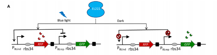
Bionetgen simulations of the blue light activated transcription matched results from the original paper and are demonstrated below.

Figure 16: Blue light simulations in Bionetgen, compared to simulations by Jayaraman et. al

To incorporate the blue light promoter/repressor into the base editing model, we simply used the concentrations of the two mRNA species as gRNA inputs for our cas9.

Figure 17: Bionetgen simulation of the base editing circuit using alternating gRNA's

While lower frequency oscillations result in less signal attenuation, the trade off is temporal resolution. With standard base editing rates, an acceptable period was found to be ~14 days (see our results page for more work on increasing base editing rates). At this timescale, the effect of regulating the base editing with a second gRNA produced a much cleaner signal in simulation, indicating the Alternating gRNA system would be a much better design choice.

Questions about Playback

How can we interpret our experimental readouts to quantify target (and off-target) base editing?

Sanger sequencing was utilized to characterize the mutation rates of each DNA frame during testing. Because our cas9 relies on only a few base pair mismatches to distinguish between frames, it was essential that we compared our on and off-target mutation frequencies. In response, we developed a python module to automatically find these sites based on binding affinities and compare the experimental data. See the CrisPy page for a detailed explanation.

Conclusion

The goal of this model was to characterize and improve the function of our CUTSCENE recording system. By developing an accurate base editing model, we were able to find ways to enhance the definition of our recording signal. During the implementation phase, we developed a method for testing our system for off-target effects. It is our hope that future teams will not only utilize our optimized recording system, but are inspired to utilize our methods for generating models and test procedures. We believe that both CrisPy and our suite of recursive bayesian estimators have the ability to succeed in real world biological applications.

References

Lillacci G, Khammash M (2010) Parameter Estimation and Model Selection in Computational Biology. PLoS Comput Biol 6(3): e1000696. doi:10.1371/journal.pcbi.1000696
Liu, Xin, and Mahesan Niranjan. “State and Parameter Estimation of the Heat Shock Response System Using Kalman and Particle Filters.” Bioinformatics, vol. 28, no. 11, 2012, pp. 1501–1507., doi:10.1093/bioinformatics/bts161.
Jayaraman, Premkumar, et al. “Blue Light-Mediated Transcriptional Activation and Repression of Gene Expression in Bacteria.” Nucleic Acids Research, vol. 44, no. 14, 2016, pp. 6994–7005., doi:10.1093/nar/gkw548.
Jeroen D. Hol, Thomas B. Schon, Fredrik Gustafsson, "ON RESAMPLING ALGORITHMS FOR PARTICLE FILTERS." Division of Automatic Control. Department of Electrical Engineering.Linkoping University. SE-581 83, Linkoping, Sweden
Harris, Leonard A., et al. “BioNetGen 2.2: Advances in Rule-Based Modeling.” Bioinformatics, vol. 32, no. 21, 2016, pp. 3366–3368., doi:10.1093/bioinformatics/btw469.
"aGrow Modeling", University of British Columnia 2017 iGEM team, https://2017.igem.org/Team:British_Columbia/Model
Farasat I, Salis HM (2016) A Biophysical Model of CRISPR/Cas9 Activity for Rational Design of Genome Editing and Gene Regulation. PLOS Computational Biology 12(1): e1004724. https://doi.org/10.1371/journal.pcbi.1004724
Farzadfard, Fahim, et al. “Single-Nucleotide-Resolution Computing and Memory in Living Cells.” BioRxiv, 2018, doi:10.1101/263657.

Team:Pittsburgh/Model