Difference between revisions of "Team:XMU-China/Model"
Cyclohexane (Talk | contribs) |
|||
| (18 intermediate revisions by 2 users not shown) | |||
| Line 1: | Line 1: | ||
| − | |||
<html lang="en"> | <html lang="en"> | ||
| Line 13: | Line 12: | ||
<meta name="keywords" content="" /> | <meta name="keywords" content="" /> | ||
<link rel="shortcut icon" href="favicon.ico" type="image/x-icon" /> | <link rel="shortcut icon" href="favicon.ico" type="image/x-icon" /> | ||
| − | <meta name="apple-touch-fullscreen" content="yes" /><!-- 是否启用 WebApp | + | <meta name="apple-touch-fullscreen" content="yes" /><!-- 是否启用 WebApp 全屏模式,删除苹果默认的工具栏和菜单栏 --> |
| − | <meta name="apple-mobile-web-app-status-bar-style" content="black" /><!-- 设置苹果工具栏颜色:默认值为 | + | <meta name="apple-mobile-web-app-status-bar-style" content="black" /><!-- 设置苹果工具栏颜色:默认值为 default,可以定为 black和 black-translucent--> |
<meta http-equiv="Cache-Control" content="no-siteapp" /><!-- 不让百度转码 --> | <meta http-equiv="Cache-Control" content="no-siteapp" /><!-- 不让百度转码 --> | ||
| − | <meta name="HandheldFriendly" content="true"><!-- | + | <meta name="HandheldFriendly" content="true"><!-- 针对手持设备优化,主要是针对一些老的不识别viewport的浏览器,比如黑莓 --> |
<meta name="MobileOptimized" content="320"><!-- 微软的老式浏览器 --> | <meta name="MobileOptimized" content="320"><!-- 微软的老式浏览器 --> | ||
<meta name="screen-orientation" content="portrait"><!-- uc强制竖屏 --> | <meta name="screen-orientation" content="portrait"><!-- uc强制竖屏 --> | ||
| Line 23: | Line 22: | ||
<meta name="x5-page-mode" content="app"><!-- QQ应用模式 --> | <meta name="x5-page-mode" content="app"><!-- QQ应用模式 --> | ||
<meta name="msapplication-tap-highlight" content="no"><!-- windows phone 点击无高光 --> | <meta name="msapplication-tap-highlight" content="no"><!-- windows phone 点击无高光 --> | ||
| − | <title>Team:XMU-China/ | + | <title>Team:XMU-China/Model - 2018.igem.org</title> |
| − | <link rel="stylesheet" href="css/ | + | <link rel="stylesheet" href="css/interlab.css"> |
| + | <link rel="dns-prefetch" href="//cdn.mathjax.org" /> | ||
| + | <link rel="dns-prefetch" href="//cdn.bootcss.com" /> | ||
<link href="http://cdn.bootcss.com/font-awesome/4.7.0/css/font-awesome.min.css" rel="stylesheet"> | <link href="http://cdn.bootcss.com/font-awesome/4.7.0/css/font-awesome.min.css" rel="stylesheet"> | ||
<link rel="stylesheet" href="https://2018.igem.org/Team:XMU-China/css/cover?action=raw&ctype=text/css"> | <link rel="stylesheet" href="https://2018.igem.org/Team:XMU-China/css/cover?action=raw&ctype=text/css"> | ||
| Line 30: | Line 31: | ||
<link rel="stylesheet" href="https://2018.igem.org/Team:XMU-China/css/nav?action=raw&ctype=text/css"> | <link rel="stylesheet" href="https://2018.igem.org/Team:XMU-China/css/nav?action=raw&ctype=text/css"> | ||
<link rel="stylesheet" href="https://2018.igem.org/Team:XMU-China/css/nav_mobile?action=raw&ctype=text/css"> | <link rel="stylesheet" href="https://2018.igem.org/Team:XMU-China/css/nav_mobile?action=raw&ctype=text/css"> | ||
| − | <link rel="stylesheet" href="https://2018.igem.org/Team:XMU-China/css/ | + | <link rel="stylesheet" href="https://2018.igem.org/Team:XMU-China/css/interlab?action=raw&ctype=text/css"> |
<link rel="stylesheet" href="https://2018.igem.org/Team:XMU-China/css/font?action=raw&ctype=text/css"> | <link rel="stylesheet" href="https://2018.igem.org/Team:XMU-China/css/font?action=raw&ctype=text/css"> | ||
<link rel="stylesheet" href="https://2018.igem.org/Team:XMU-China/css/material-scrolltop?action=raw&ctype=text/css"> | <link rel="stylesheet" href="https://2018.igem.org/Team:XMU-China/css/material-scrolltop?action=raw&ctype=text/css"> | ||
| Line 36: | Line 37: | ||
<body> | <body> | ||
| + | <header></header> | ||
<div id="container"> | <div id="container"> | ||
<header> | <header> | ||
| Line 46: | Line 48: | ||
<li><a href="https://2018.igem.org/Team:XMU-China/Description">Description</a></li> | <li><a href="https://2018.igem.org/Team:XMU-China/Description">Description</a></li> | ||
<li><a href="https://2018.igem.org/Team:XMU-China/Design">Design</a></li> | <li><a href="https://2018.igem.org/Team:XMU-China/Design">Design</a></li> | ||
| − | |||
<li><a href="https://2018.igem.org/Team:XMU-China/Results">Results</a></li> | <li><a href="https://2018.igem.org/Team:XMU-China/Results">Results</a></li> | ||
| + | <li><a href="https://2018.igem.org/Team:XMU-China/Demonstrate">Demonstrate</a></li> | ||
<li><a href="https://2018.igem.org/Team:XMU-China/Parts">Parts</a></li> | <li><a href="https://2018.igem.org/Team:XMU-China/Parts">Parts</a></li> | ||
</ul> | </ul> | ||
| Line 57: | Line 59: | ||
<ul> | <ul> | ||
<li><a href="https://2018.igem.org/Team:XMU-China/Hardware">Overview</a></li> | <li><a href="https://2018.igem.org/Team:XMU-China/Hardware">Overview</a></li> | ||
| − | <li><a href="https://2018.igem.org/Team:XMU-China/Hardware | + | <li><a href="https://2018.igem.org/Team:XMU-China/Hardware#Microfluidic_Chips">Microfluidic Chips</a></li> |
| − | <li><a href="https://2018.igem.org/Team:XMU-China/Hardware | + | <li><a href="https://2018.igem.org/Team:XMU-China/Hardware#Fluorescence_Detection">Fluorescence Detection</a></li> |
| − | <li><a href="https://2018.igem.org/Team:XMU-China/Hardware | + | <li><a href="https://2018.igem.org/Team:XMU-China/Hardware#Raspberry_Pi">Raspberry Pi</a></li> |
| − | <li><a href="https://2018.igem.org/Team:XMU-China/ | + | <li><a href="https://2018.igem.org/Team:XMU-China/Hardware#Application">Application</a></li> |
| − | <li><a href="https://2018.igem.org/Team:XMU-China/Software"> | + | <li><a href="https://2018.igem.org/Team:XMU-China/Software">Software</a></li> |
| + | <li><a href="https://2018.igem.org/Team:XMU-China/Applied_Design">Product Design</a></li> | ||
</ul> | </ul> | ||
</li> | </li> | ||
| Line 67: | Line 70: | ||
<a href="#">Model</a> | <a href="#">Model</a> | ||
<ul> | <ul> | ||
| − | <li><a href="https://2018.igem.org/Team:XMU-China/Model"> | + | <li><a href="https://2018.igem.org/Team:XMU-China/Model#Summary">Summary</a></li> |
| + | <li><a href="https://2018.igem.org/Team:XMU-China/Model#Thermodynamic_model">Thermodynamic Model</a></li> | ||
| + | <li><a href="https://2018.igem.org/Team:XMU-China/Model#Fluid_dynamics_model">Fluid dynamics Model</a></li> | ||
| + | <li><a href="https://2018.igem.org/Team:XMU-China/Model#Molecular_docking_model">Molecular Docking Model</a></li> | ||
| + | <li><a href="https://2018.igem.org/Team:XMU-China/Model#The_dynamic_model">Derivation of Rate Equation</a></li> | ||
</ul> | </ul> | ||
</li> | </li> | ||
<li class="Human_Practice"> | <li class="Human_Practice"> | ||
| − | <a href="#"> | + | <a href="#">Social Works</a> |
<ul> | <ul> | ||
<li><a href="https://2018.igem.org/Te | <li><a href="https://2018.igem.org/Te | ||
| − | am:XMU-China/Human_Practices"> | + | am:XMU-China/Human_Practices">Human Practice</a></li> |
| − | + | ||
| − | + | ||
<li><a href="https://2018.igem.org/Team:XMU-China/Public_Engagement">Engagement</a></li> | <li><a href="https://2018.igem.org/Team:XMU-China/Public_Engagement">Engagement</a></li> | ||
<li><a href="https://2018.igem.org/Team:XMU-China/Collaborations">Collaborations</a></li> | <li><a href="https://2018.igem.org/Team:XMU-China/Collaborations">Collaborations</a></li> | ||
| Line 96: | Line 101: | ||
<li><a href="https://2018.igem.org/Team:XMU-China/Notebook">Notebook</a></li> | <li><a href="https://2018.igem.org/Team:XMU-China/Notebook">Notebook</a></li> | ||
<li><a href="https://2018.igem.org/Team:XMU-China/Experiments">Experiments</a></li> | <li><a href="https://2018.igem.org/Team:XMU-China/Experiments">Experiments</a></li> | ||
| + | <li><a href="https://2018.igem.org/Team:XMU-China/Engineering">Engineering</a></li> | ||
</ul> | </ul> | ||
</li> | </li> | ||
| Line 104: | Line 110: | ||
<li><a href="https://2018.igem.org/Team:XMU-China/Attributions">Attributions</a></li> | <li><a href="https://2018.igem.org/Team:XMU-China/Attributions">Attributions</a></li> | ||
<li><a href="https://2018.igem.org/Team:XMU-China/Judging">Judging</a></li> | <li><a href="https://2018.igem.org/Team:XMU-China/Judging">Judging</a></li> | ||
| + | <li><a href="https://2018.igem.org/Team:XMU-China/After_iGEM">After iGEM</a></li> | ||
</ul> | </ul> | ||
</li> | </li> | ||
| Line 113: | Line 120: | ||
</div> | </div> | ||
<script src="js/jquery-1.11.0.min.js"></script> | <script src="js/jquery-1.11.0.min.js"></script> | ||
| − | |||
<script src="https://2018.igem.org/Team:XMU-China/js/hc-mobile-nav?action=raw&ctype=text/javascript"></script> | <script src="https://2018.igem.org/Team:XMU-China/js/hc-mobile-nav?action=raw&ctype=text/javascript"></script> | ||
<div class="header"> | <div class="header"> | ||
| Line 128: | Line 134: | ||
<li><a href="https://2018.igem.org/Team:XMU-China/Attributions">Attributions</a></li> | <li><a href="https://2018.igem.org/Team:XMU-China/Attributions">Attributions</a></li> | ||
<li><a href="https://2018.igem.org/Team:XMU-China/Judging">Judging</a></li> | <li><a href="https://2018.igem.org/Team:XMU-China/Judging">Judging</a></li> | ||
| + | <li><a href="https://2018.igem.org/Team:XMU-China/After_iGEM">After iGEM</a></li> | ||
</ul> | </ul> | ||
</div> | </div> | ||
<div id="Notebook"> | <div id="Notebook"> | ||
| − | + | <div class="nav-word">Notebook</div> | |
| − | + | ||
| − | + | ||
<ul> | <ul> | ||
<li><a href="https://2018.igem.org/Team:XMU-China/Notebook">Notebook</a></li> | <li><a href="https://2018.igem.org/Team:XMU-China/Notebook">Notebook</a></li> | ||
<li><a href="https://2018.igem.org/Team:XMU-China/Experiments">Experiments</a></li> | <li><a href="https://2018.igem.org/Team:XMU-China/Experiments">Experiments</a></li> | ||
| + | <li><a href="https://2018.igem.org/Team:XMU-China/Engineering">Engineering</a></li> | ||
</ul> | </ul> | ||
</div> | </div> | ||
| Line 149: | Line 155: | ||
</div> | </div> | ||
<div id="Human_Practice"> | <div id="Human_Practice"> | ||
| − | <div class="nav-word"> | + | <div class="nav-word">Social Works</div> |
<ul> | <ul> | ||
| − | <li><a href="https://2018.igem.org/Team:XMU-China/Human_Practices"> | + | <li><a href="https://2018.igem.org/Team:XMU-China/Human_Practices">Human Practice</a></li> |
| − | + | ||
| − | + | ||
<li><a href="https://2018.igem.org/Team:XMU-China/Public_Engagement">Engagement</a></li> | <li><a href="https://2018.igem.org/Team:XMU-China/Public_Engagement">Engagement</a></li> | ||
<li><a href="https://2018.igem.org/Team:XMU-China/Collaborations">Collaborations</a></li> | <li><a href="https://2018.igem.org/Team:XMU-China/Collaborations">Collaborations</a></li> | ||
| Line 162: | Line 166: | ||
<div class="nav-word">Model</div> | <div class="nav-word">Model</div> | ||
<ul> | <ul> | ||
| − | <li><a href="https://2018.igem.org/Team:XMU-China/Model"> | + | <li><a href="https://2018.igem.org/Team:XMU-China/Model">Summary</a></li> |
| + | <li><a href="https://2018.igem.org/Team:XMU-China/Model#Thermodynamic_model">Thermodynamic Model</a></li> | ||
| + | <li><a href="https://2018.igem.org/Team:XMU-China/Model#Fluid_dynamics_model">Fluid dynamics Model</a></li> | ||
| + | <li><a href="https://2018.igem.org/Team:XMU-China/Model#Molecular_docking_model">Molecular Docking Model</a></li> | ||
| + | <li><a href="https://2018.igem.org/Team:XMU-China/Model#The_dynamic_model">Derivation of Rate Equation</a></li> | ||
</ul> | </ul> | ||
</div> | </div> | ||
| Line 169: | Line 177: | ||
<ul> | <ul> | ||
<li><a href="https://2018.igem.org/Team:XMU-China/Hardware">Overview</a></li> | <li><a href="https://2018.igem.org/Team:XMU-China/Hardware">Overview</a></li> | ||
| − | <li><a href="https://2018.igem.org/Team:XMU-China/Hardware | + | <li><a href="https://2018.igem.org/Team:XMU-China/Hardware#Microfluidic_Chips">Microfluidic Chips</a></li> |
| − | <li><a href="https://2018.igem.org/Team:XMU-China/Hardware | + | <li><a href="https://2018.igem.org/Team:XMU-China/Hardware#Fluorescence_Detection">Fluorescence Detection</a></li> |
| − | <li><a href="https://2018.igem.org/Team:XMU-China/Hardware | + | <li><a href="https://2018.igem.org/Team:XMU-China/Hardware#Raspberry_Pi">Raspberry Pi</a></li> |
| − | <li><a href="https://2018.igem.org/Team:XMU-China/ | + | <li><a href="https://2018.igem.org/Team:XMU-China/Hardware#Application">Application</a></li> |
| − | <li><a href="https://2018.igem.org/Team:XMU-China/Software"> | + | <li><a href="https://2018.igem.org/Team:XMU-China/Software">Software</a></li> |
| + | <li><a href="https://2018.igem.org/Team:XMU-China/Applied_Design">Product Design</a></li> | ||
</ul> | </ul> | ||
</div> | </div> | ||
| Line 181: | Line 190: | ||
<li><a href="https://2018.igem.org/Team:XMU-China/Description">Description</a></li> | <li><a href="https://2018.igem.org/Team:XMU-China/Description">Description</a></li> | ||
<li><a href="https://2018.igem.org/Team:XMU-China/Design">Design</a></li> | <li><a href="https://2018.igem.org/Team:XMU-China/Design">Design</a></li> | ||
| − | |||
<li><a href="https://2018.igem.org/Team:XMU-China/Results">Results</a></li> | <li><a href="https://2018.igem.org/Team:XMU-China/Results">Results</a></li> | ||
| + | <li><a href="https://2018.igem.org/Team:XMU-China/Demonstrate">Demonstrate</a></li> | ||
<li><a href="https://2018.igem.org/Team:XMU-China/Parts">Parts</a></li> | <li><a href="https://2018.igem.org/Team:XMU-China/Parts">Parts</a></li> | ||
</ul> | </ul> | ||
| Line 195: | Line 204: | ||
<div class="clear"></div> | <div class="clear"></div> | ||
<div class="description_banner"> | <div class="description_banner"> | ||
| − | <div class="word"> | + | <div class="word">Model</div> |
</div> | </div> | ||
<nav class="Quick-navigation"> | <nav class="Quick-navigation"> | ||
<div class="Quick-navigation_word"> | <div class="Quick-navigation_word"> | ||
| − | <img src="https://static.igem.org/mediawiki/2018/ | + | <img src="https://static.igem.org/mediawiki/2018/e/e6/T--XMU-China--right50.png"> |
| − | <a href="# | + | <a href="#Summary" class="Quick-navigation-item"> |
| − | <img id="turn_img" src="https://static.igem.org/mediawiki/2018/ | + | <img id="turn_img" src="https://static.igem.org/mediawiki/2018/5/50/T--XMU-China--right51.png"> |
| − | <a href="# | + | <a href="#Summary"id="Quick_A">Summary</a></a> |
| − | <a href="# | + | <a href="#Thermodynamic_model" class="Quick-navigation-item" > |
| − | <img id="turn_img" src="https://static.igem.org/mediawiki/2018/ | + | <img id="turn_img" src="https://static.igem.org/mediawiki/2018/0/04/T--XMU-China--right52.png"> |
| − | <a href="# | + | <a href="#Thermodynamic_model" id="Quick_B">Thermodynamic model</a></a> |
| − | <a href="# | + | <a href="#Fluid_dynamics_model" class="Quick-navigation-item"> |
| − | <img id="turn_img" src="https://static.igem.org/mediawiki/2018/ | + | <img id="turn_img" src="https://static.igem.org/mediawiki/2018/d/d0/T--XMU-China--right53.png"> |
| − | <a href="# | + | <a href="#Fluid_dynamics_model" id="Quick_C">Fluid dynamics model</a></a> |
| + | <a href="#Molecular_docking_model" class="Quick-navigation-item"> | ||
| + | <img id="turn_img" src="https://static.igem.org/mediawiki/2018/1/11/T--XMU-China--right54.png"> | ||
| + | <a href="#Molecular_docking_model"id="Quick_D">Molecular docking model</a></a> | ||
| + | <a href="#The_dynamic_model" class="Quick-navigation-item"> | ||
| + | <img id="turn_img" src="https://static.igem.org/mediawiki/2018/b/ba/T--XMU-China--right55.png"> | ||
| + | <a href="#The_dynamic_model"id="Quick_F">Derivation of rate equation | ||
| + | </a></a> | ||
</div> | </div> | ||
</nav> | </nav> | ||
| − | <div class="main"> | + | <div class="main" id="post-content"> |
| − | <section id=" | + | <section id="Summary" class="js-scroll-step"> |
<div class="headline"> | <div class="headline"> | ||
| − | + | Summary | |
</div> | </div> | ||
| − | + | ||
| − | <p> | + | <p class="indent">Based on the hypothesis of nearest neighbor method and the dissociation constant of aptamer-"complementary strand" complex, starting from the aspect of thermodynamics, we focused on the change of standard Gibbs free energy to construct "ABKey function" about upper limit of the length of complementary sequence, then we obtained the upper limit by invoking the function to assist in narrowing the choice range of our experimental materials. In order to avoid false positive of dissociation of our aptamer and "complementary strand" designed under the impact of the flow, we constructed fluid dynamic model to check whether our designed rotating speed is viable or not based on the dimension homogeneous principle. In this model, we gave out a feasible rotating speed by utilizing an elementary analysis method--dimensional analysis method to instruct the hardware. Modeling is not only reflected in numbers, but the vividness of images is also an important advantage of modeling. We used multiple softwares to build 3D simulation models of protein, RNA and DNA, one after another. Then we carried out the molecular docking between the DNA and protein, which provided critical basis and help for the subsequent experiments. Besides, we constructed the dynamics model of the competitive reaction using differential equations to derivate the rate equation of particular competitive reaction with the exact method of verification through experiment given as well. |
| + | |||
</p> | </p> | ||
| − | <p> | + | </section> |
| + | <section id="Thermodynamic_model" class="js-scroll-step"> | ||
| + | <div class="headline"> | ||
| + | Thermodynamic Model | ||
| + | </div> | ||
| + | <p class="indent">The strength of the binding between the aptamer (A) and its target protein (P) can be described by dissociation constant K$^{\circ}_{d1}$: | ||
| + | $$AP\rightleftharpoons A+P \qquad K^{\circ}_{d1}=\frac{[A][P]}{[AP]}$$ | ||
</p> | </p> | ||
| − | <p> | + | <p>It is assumed that a similar dissociation constant exists for the aptamer (A) and its "complementary strand"(C) K$^{\circ}_{d2}$: |
| + | $$AC\rightleftharpoons A+C \qquad K^{\circ}_{d2}=\frac{[A][C]}{[AC]}$$ | ||
</p> | </p> | ||
| − | <p> | + | <p>The equation for the competitive reaction is |
| + | $$AC+P\rightleftharpoons AP+C \qquad K^{\circ}=\frac{K^{\circ}_{d2}}{K^{\circ}_{d1}}$$ | ||
</p> | </p> | ||
| − | <p | + | <p> |
| − | + | In order to compete spontaneously in the forward direction, the equilibrium constant K$^{\circ}$ must satisfy condition that K$^{\circ}>$1, which means K$^{\circ}_{d2}>$K$^{\circ}_{d1}$. The EpCAM protein and its aptamer(SYL3C) were taken as an example, and the compound's dissociation constant$^{[1]}$ is $(22.8\pm6.0)\times10^{-9}$mol/L, so K$^{\circ}_{d2}>28.8\times10^{-9}$mol/L. | |
| − | + | ||
</p> | </p> | ||
| − | |||
| − | |||
| − | |||
<p> | <p> | ||
| − | + | The assumption of nearest neighbor method$^{[2]}$: | |
| − | + | ||
| − | + | ||
| − | + | ||
| − | + | ||
| − | + | ||
| − | + | ||
| − | + | ||
| − | + | ||
| − | + | ||
| − | + | ||
| − | + | ||
</p> | </p> | ||
| + | <p>$\bullet$The initial concentration of two single nucleic acid chains in the hybridization reaction is the same;</p> | ||
| + | <p>$\bullet$The nucleic acid hybridization reaction satisfies the distate model, i.e., the dechain and the formation of the double strand are always dynamically balanced;</p> | ||
| + | <p>$\bullet$The hybrid nucleic acid double strand is a single double helix structure.</p> | ||
| + | <p>The nearest neighbor method is that changing the standard free energy of the hybridization process of DNA molecules into the summation($\Sigma_{i}$n$_{i}$$\triangle $G$^{\circ}$(i)) of the standard free energy of the 10 dimers(Duplex) formed by the four bases(A, G, C, T) that make up the DNA molecules, then plus the starting or ending base pairs of DNA moleculesGC, AT($\triangle$G$^{\circ}$(init.w/term.G$\cdot$C), $\triangle$G$^{\circ}$(init.w/term.A$\cdot$T)) and the effects of factors such as sequence symmetry ($\triangle$G$^{\circ}$(Sym)), as well as the salt concentration of correction. The data of standard gibbs free energy change of ten dimers are shown in the following table: (1 cal = 4.1859 J)</p> | ||
| + | <p> | ||
| + | $$\begin{array}{|c|c|c|c|c|c|c|}\hline | ||
| + | Sequence & AA/TT & AT/TA & TA/AT & CA/GT & GT/CA & CT/GA \\\hline | ||
| + | Parameter,kcal/mol & -1.00 & -0.88 & -0.58 & -1.45 & -1.44 & -1.28 \\\hline | ||
| + | Sequence & GA/CT & CG/GC & GC/CG & GG/CC & init.w/term.G \cdot C &init.w/term.A \cdot T\\\hline | ||
| + | Parameter,kcal/mol & -1.30 & -2.17 & -2.24 & -1.84 & 0.98 & 1.03 \\ | ||
| + | \hline \end{array}$$ | ||
| + | </p> | ||
| + | <p>According to "nearest neighbor method", $A+C\rightleftharpoons AC$(K$^{\circ}$=$\frac{1}{K^{\circ}_{d2}})$, Standard Free Energy Change $\triangle$G$^{\circ}$ = $\triangle$G$^{\circ}$(total) - 0.175$\cdot$$\ln$[Na$^{+}$] - 0.20, and $\triangle$G$^{\circ}$(total)=$\Sigma_{i}$n$_{i}$$\triangle$G$^{\circ}$(i)+$\triangle$G$^{\circ}$ (init.w/term.G$\cdot$C)+ $\triangle$G$^{\circ}$ (init.w/term.A$\cdot$T)+ $\triangle$G$^{\circ}$(Sym).</p> | ||
| + | <p>The sequence of aptamer SYL3C is: 5' - CAC TAC AGA GGT TGC GTC TGT CCC ACG TTG TCA TGG GGG GTT GGC CTG - 3'. Since the 3' port is fixed on the solid base, only the 5' port can be moved.</p> | ||
| + | <p>The data used at this time is as follows:</p> | ||
| + | <p> | ||
| + | $$\begin{array}{|c|c|c|c|c|c|c|}\hline | ||
| + | % after \\: \hline or \cline{col1-col2} \cline{col3-col4} ... | ||
| + | Sequence & Parameter(kcal/mol) \\\hline | ||
| + | AA &-1.00 \\ | ||
| + | AC & -1.44 \\ | ||
| + | AG& -1.28 \\ | ||
| + | AT &-0.88 \\ | ||
| + | CA & -1.45 \\ | ||
| + | CC& -1.84 \\ | ||
| + | CG &-2.17 \\ | ||
| + | CT & -1.28 \\ | ||
| + | GA& -1.30 \\ | ||
| + | GC &-2.24 \\ | ||
| + | GG & -1.84 \\ | ||
| + | GT& -1.44 \\ | ||
| + | TA &-0.58 \\ | ||
| + | TC & -1.30 \\ | ||
| + | TG& -1.45 \\ | ||
| + | TT &-1.00 \\ | ||
| + | init.w/term.G \cdot C & 0.98 \\ | ||
| + | init.w/term.A \cdot T & 1.03 \\ | ||
| + | \hline | ||
| + | \end{array}$$ | ||
| + | </p> | ||
| + | <p>Using self-defined "ABKey function" for this chain, then we get the upper limit 10.</p> | ||
| + | <p class="F3"> | ||
| + | <img src="https://static.igem.org/mediawiki/2018/c/ce/T--XMU-China--model-answer.png"> | ||
| + | <p class="Figure_word"> | ||
| + | <strong>Figure 1</strong>: ANSWER | ||
| + | </p> | ||
| + | </p> | ||
| + | <p>Simple flow chart of the "ABKey function"</p> | ||
| + | <p class="F3"> | ||
| + | <img src="https://static.igem.org/mediawiki/2018/6/6d/T--XMU-China--model-flow.png"> | ||
| + | <p class="Figure_word"> | ||
| + | <strong>Figure 2</strong>: Chain length upper limit selection mechanism | ||
| + | </p> | ||
| + | </p> | ||
| + | <p>Equation set of the ABKey function:</p> | ||
| + | <p>\begin{equation*} | ||
| + | \begin{cases} | ||
| + | \triangle G^{\circ}=\Sigma_{i} \triangle G_{i}^{\circ}\\ | ||
| + | \triangle G^{\circ}=- RT\ln K^{\circ}\\ | ||
| + | K_{d}=\frac{1}{K^{\circ}}\\ | ||
| + | K_{d}\geq \widetilde{K_{d}}=28.8\times10^{-9}mol/L | ||
| + | \end{cases} | ||
| + | \end{equation*} | ||
| + | </p> | ||
| + | <p>In fact, the number 10 happens to be a critical value. From 10 bases down, 9 or 8 base complements can also cause "competition" to occur spontaneously in the forward direction, but the fewer the complementary bases, the less likely it is that the aptamer - "complementary strand" double chain structure can be formed, resulting in the loss of the basis of "competition".</p> | ||
| + | <p class="F3"> | ||
| + | <img src="https://static.igem.org/mediawiki/2018/d/d9/T--XMU-China--model-line.png"> | ||
| + | <p class="Figure_word"><strong>Figure 3</strong>: Line Chart</p> | ||
| + | </p> | ||
| + | <p>On the other hand, the minimum complementary value was set as 5 according to the | ||
| + | literature.</p> | ||
| + | <h1>References</h1> | ||
| + | <p class="reference">[1] JOHN SANTALUCIA, JR*, A unified view of polymer, dumbbell, and oligonucleotide DNA nearest-neighbor thermodynamics, <i>Proc Natl Acad Sci Anal Chem</i>, <strong>1998</strong>, 95, 1460-1465.<br> | ||
| + | [2] Yanling Song, Zhi Zhu, Yuan An, Weiting Zhang, Huimin Zhang, Dan Liu, Chundong | ||
| + | Yu, Wei Duan, Chaoyong James Yang, Selection of DNA Aptamers against Epithelial Cell | ||
| + | Adhesion Molecule for Cancer Cell Imaging and Circulating Tumor Cell Capture, <i>Proc Natl Acad Sci Anal Chem</i>, <strong>2013</strong>, 85, 4141-4149.</p> | ||
</section> | </section> | ||
| − | <section id=" | + | <section id="Fluid_dynamics_model" class="js-scroll-step"> |
<div class="headline"> | <div class="headline"> | ||
| − | + | Fluid Dynamics Model | |
</div> | </div> | ||
| − | + | <p>In order to ensure that the adaptor and the complementary sequence designed by us are | |
| − | <p> | + | not dissociated continuously under the impact of the liquid, which leads to false positive results, |
| + | our modeling guides us to determine whether the designed rotation speed is reasonable. | ||
</p> | </p> | ||
| − | <p | + | <p>Referring to the knowledge of chemical fluid flow and DNA structure, we designed a model |
| − | + | that guided us to calculate the maximum rotational speed or maximum pressure difference | |
| − | + | under overall stability between the aptamer and complementary sequences. It's crucial to the | |
| + | hardware. | ||
</p> | </p> | ||
| + | <p>First, we focused on the relation between the flow velocity and rotation speed in the | ||
| + | pipeline driven by centrifugal force only. Under the condition of laminar flow, we introduced | ||
| + | several assumptions:</p> | ||
| + | <p>1. Ignoring the effects of gravity; </p> | ||
| + | <p>2. Ignoring the problem of force distribution in the vertical direction, and considered it as the uniform distribution;</p> | ||
| + | <p>3. As both ends of the fluid passed through the atmosphere, the pressure difference between the two ends of the fluid was ignored.</p> | ||
| + | <p>Based on the above hypothesis, the specific principle content and derivation are as follows:</p> | ||
| + | <p>The general formula of steady-state flow friction resistance of fluid in fluid mechanics is as | ||
| + | follows: | ||
| + | </p> | ||
| + | <p>\begin{equation} | ||
| + | (p_{1}-p_{2})\pi r^{2}= \tau 2\pi rL \tag{2.1} | ||
| + | \end{equation} | ||
| + | </p> | ||
| + | <p>Then, in the same way as the settlement hypothesis, we introduced the fourth hypothesis: | ||
| + | the fluid accelerates in the pipe for a short time, and the whole process is considered to be | ||
| + | uniform.</p> | ||
| + | <p>According to the force analysis, when the fluid flows outward because of centrifugal, there | ||
| + | is no pressure difference, and only the centripetal force is provided by the resistance, i.e.</p> | ||
| + | <p>\begin{equation} | ||
| + | \tau 2\pi rL= F_{x} \tag{2.2} | ||
| + | \end{equation} | ||
| + | </p> | ||
| + | <p>At the same time, the flow velocity is usually reflected in the pressure drop, so we can | ||
| + | combine (2.1) and (2.2), and relate the centripetal force $F_{x}$ to the pressure drop, and then show its | ||
| + | effect on the flow rate. That is:</p> | ||
| + | <p>\begin{equation} | ||
| + | (p_{1}-p_{2})\pi r^{2}= F_{x} \tag{2.3} | ||
| + | \end{equation} | ||
| + | </p> | ||
| + | <p>What's more,</p> | ||
| + | <p>\begin{equation} | ||
| + | F_{x}=m\omega ^{2}R= 4\pi ^{2}mn^{2}R \tag{2.4} | ||
| + | \end{equation} | ||
| + | </p> | ||
| + | <p>\begin{equation} | ||
| + | m= \rho \pi r^{2}L \tag{2.5} | ||
| + | \end{equation} | ||
| + | </p> | ||
| + | <p>From equations (2.3), (2.4) and (2.5), we can obtain the relation between pressure drop and flow velocity:</p> | ||
| + | |||
| + | <p>\begin{equation} | ||
| + | \Delta p_{sf}=4\pi ^{2}n ^{2}\rho LR \tag{2.6} | ||
| + | \end{equation} | ||
| + | where $\tau$(Pa) represents the friction force, $\rho$(kg/m$^{3}$) represents the fluid density, n(r/s) represents the rotation speed, L(m) represents the fluid length, R(m) represents the length of fluid center to center of circle, r(m) represents radius of circular tube. For a variety of tubes, we can use different correction coefficients or hydraulic diameters to convert the tube diameter, but the tube shape is only reflected in r, and the r in the formula is also eliminated. Therefore, we considered equation (2.6) to be valid for any tube shape and theoretically free of error.</p> | ||
| + | <p>Then, because our fluid motion was carried out in the rectangular tube and is laminar | ||
| + | flow, we can use the laminar flow relationship between pressure drop and flow velocity in the | ||
| + | rectangular section pipe:</p> | ||
| + | <p>\begin{equation} | ||
| + | \Delta p_{sf}=\frac{12\mu u_{b}L}{b^{2}}[1-\frac{192b}{\pi ^{5}a}th(\frac{\pi a}{2b})]^{-1} \tag{2.7} | ||
| + | \end{equation} | ||
| + | </p> | ||
| + | <p>By substituting equation (2.7) into equation (2.6), we obtained the laminar flow relationship | ||
| + | between the speed and the flow velocity in the rectangular pipeline:</p> | ||
| + | <p>\begin{equation} | ||
| + | u_{b}=\frac{4\pi ^{2}\rho b^{2}R}{12\mu}[1-\frac{192b}{\pi ^{5}a}th(\frac{\pi a}{2b})]\ast n^{2} \tag{2.8} | ||
| + | \end{equation} | ||
| + | </p> | ||
| + | <p>In the above, a(m) is the long side length of rectangular section pipeline and b(m) is the | ||
| + | short side length.</p> | ||
| + | <p>At this point, we have completed the derivation of the first part about the relation between | ||
| + | flow velocity and rotation speed.</p> | ||
| + | <p>The second part is to derive the relationship between drag force and flow velocity. Also | ||
| + | under the condition of laminar flow, we introduced the following assumptions: | ||
| + | </p> | ||
| + | <p>1.During the process, the fluid’s force on the solid is provided by the drag force; | ||
| + | </p> | ||
| + | <p>2.No head loss is considered during liquid flow.</p> | ||
| + | <p>In the process of particle deposition, the drag equation is very consistent with the impact | ||
| + | process of our fluid on DNA. The formula is as follows:</p> | ||
| + | <p>\begin{equation} | ||
| + | F_{d}=\zeta A\frac{\rho u_{t}^{2}}{2} \tag{2.9} | ||
| + | \end{equation} | ||
| + | </p> | ||
| + | <p>In formula (2.9), $\zeta$ represents the drag coefficient with a dimension of 1; A(m$^{2}$) represents the movement of fluid's flowing through the plane area; $\rho$(kg/m$^{3}$) represents fluid density; $u_{t}$(m/s) represents the velocity of the particle relative to the fluid.</p> | ||
| + | <p>In laminar flow, the correlation between $\zeta$ and relative motion Reynolds number Ret and relative motion Reynolds number Ret is defined as:</p> | ||
| + | <p>\begin{equation} | ||
| + | \zeta =\frac{24}{Re_{t}} \tag{2.10} | ||
| + | \end{equation} | ||
| + | </p> | ||
| + | <p>\begin{equation} | ||
| + | Re_{t}=\frac{d_{s}u_{t}\rho }{\mu } \tag{2.11} | ||
| + | \end{equation} | ||
| + | </p> | ||
| + | <p>Substitute (2.10) and (2.11) into equation (2.9) and we have:</p> | ||
| + | <p>\begin{equation} | ||
| + | F_{d}=\frac{12\mu u_{t}A}{d_{s}} \tag{2.12} | ||
| + | \end{equation} | ||
| + | </p> | ||
| + | <p>In equation (2.12), ds represents the diameter or equivalent diameter of particles. A is also | ||
| + | related to ds. And because DNA is a double helix structure, the error in equivalent diameters | ||
| + | is huge. Therefore, by simplifying the calculation of A, we want to keep A and get rid of ds.</p> | ||
| + | <p>There is Stokes Law in laminar flow:</p> | ||
| + | <p>\begin{equation} | ||
| + | F_{d}=3\pi \mu u_{t}d_{s}\tag{2.13} | ||
| + | \end{equation} | ||
| + | </p> | ||
| + | <p>By combining equations (2.12) and (2.13), the final formula of traction can be obtained:</p> | ||
| + | <p>\begin{equation} | ||
| + | F_{d}=\sqrt{36\pi A}\mu u_{t} \tag{2.14} | ||
| + | \end{equation} | ||
| + | where $\mu$ represents the viscosity of the fluid.</p> | ||
| + | <p>In addition, $u_{t}$ represents the velocity of the particle relative to the fluid. Since our adaptor is fixed on the plane, $u_{t}$=$u_{b}$(fluid velocity).</p> | ||
| + | <p>The third part is the dna-related model. To simplify the model, we introduced the following assumptions:</p> | ||
| + | <p>1.Simplified DNA molecular model, the flow through DNA as a rectangle, ignoring three- | ||
| + | dimensional structure; | ||
| + | <p>2.The simplified DNA model is supposed to be B-DNA and the base pair is WC pairing; | ||
| + | </p> | ||
| + | <p>3.The base pair is considered to be completely dissociated after being destroyed by impact; | ||
| + | </p> | ||
| + | <p>4.The forces between the stable DNA consider only the hydrogen bond between base pairs.</p> | ||
| + | </p> | ||
| + | <p>Following second part, we can use the DNA molecular structure to figure out the projected area A of the moving plane through which the fluid flows.</p> | ||
<p class="F2"> | <p class="F2"> | ||
| − | <img src="https://static.igem.org/mediawiki/2018/ | + | <img src="https://static.igem.org/mediawiki/2018/e/e2/T--XMU-China--model-001.png"> |
| − | <p class="Figure_word">Figure 3 | + | <p class="Figure_word"> |
| + | <strong>Figure 1</strong>: come from wiki <sup>[3]</sup> | ||
| + | </p> | ||
</p> | </p> | ||
| − | + | <p>We chose a most common B - DNA as a model. The distance that per chain of the double helix chains having a full circle around the axis (360$\eta$$^{\circ}$) up (or down) is 3.57 nm, usually containing 10.5 nucleotide. Therefore, each two adjacent base’s flat vertical distance is 0.34 nm. And the space between two chains are also certain, i.e., 2 nm.</p> | |
| − | + | <p>Then, we have</p> | |
| + | <p>\begin{equation} | ||
| + | A= \frac{0.34\ast 10^{-9}\ast 2\ast 10^{-9}\ast n}{2} \tag{2.15} | ||
| + | \end{equation} | ||
| + | </p> | ||
| + | <p>In equation (2.15), A represents the area of the base pair through which the fluid flows, and n represents the nucleotide number used to activate crRNA. Because once the designed crRNA is determined, n is constant. So A is constant.</p> | ||
| + | <p>After finding the area A, we substitute it into equation (2.14), and the work of the total traction force can be obtained by the formula of force and work:</p> | ||
| + | <p>\begin{equation} | ||
| + | W_{d}=F_{d}\ast \Delta x \tag{2.16} | ||
| + | \end{equation} | ||
| + | </p> | ||
| + | <p>Later, we obtained the following information in some literatures:</p> | ||
| + | <p>The two hydrogen bonds of the AT base pair basically break at the same time, and the three hydrogen bonds of the CG base pair break one by one. To prevent them from being swept away, what we need to consider is their energy barrier: the simultaneous breaking energy barrier of AT base pair is 23 KJ$\cdot$mol$^{-1}$, and CG base pair maximum energy barrier, namely the first hydrogen bond breaking threshold, is also 23 KJ$\cdot$mol$^{-1}$. So we can average out the base pairs at 23 KJ$\cdot$mol $^{-1}$ per base pair.</p> | ||
| + | <p>The distance between two hydrogen bonds that break AT base pairs is $\Delta$x$_{1}$=0.74-0.63=0.11nm; The distance to break the first hydrogen bond of the CG base is $\Delta$x$_{2}$= 0.72-0.65=0.07 nm.$^{[2]}$</p> | ||
| + | <p>We took the larger $\Delta$x as the fixed value of $\Delta$x, because the bigger the $\Delta$x gets, the more work it does.</p> | ||
| + | <p>Combining the three parts, we used the fluid dynamics model to guide our hardware design. At the same time, in order to ensure that there is no dissociation, we took the maximum energy barrier of a single base pair for conversion. Therefore, the rotation speed was independent from the complementary number.</p> | ||
| + | <p>We have simultaneous equations (2.8), (2.14), (2.15) and (2.16), and the final formula is:</p> | ||
| + | <p>\begin{equation} | ||
| + | W_{d}=\frac{11}{300}\ast 10^{-18}\ast \sqrt{\frac{306\pi ^{5}k}{25}}\ast \rho b^{2}R\ast [1-\frac{192b}{\pi ^{5}a}th(\frac{\pi a}{2b})]\ast n^{2} \tag{2.17} | ||
| + | \end{equation} | ||
| + | </p> | ||
| + | <p>The above equation is substituted into the calculation equation</p> | ||
| + | <p>\begin{equation} | ||
| + | W_{d}=\frac{11}{300}\ast 10^{-18}\ast \sqrt{\frac{306\pi ^{5}k}{25}}\ast \rho b^{2}R\ast [1-\frac{192b}{\pi ^{5}a}th(\frac{\pi a}{2b})]\ast n^{2}\leq \frac{23\ast 10^{3}}{6.022\ast 10^{23}} \tag{2.18} | ||
| + | \end{equation} | ||
| + | where k represents the number of nucleotides used to activate crRNA; $\rho$(kg/m $^ {3} $) represents fluid density, which is almost equal to the density of water; a(m) represents long side length of rectangular pipeline; b(m) represents short side length; R(m) represents the length from the fluid center to the center of the circle, which, in our hardware, is the length of the coating center to the center of the circle; n(r/s) represents rotation speed.</p> | ||
| + | <p>In our hardware design, a=b=1mm; k=21; $\rho$ is approximately equal to the density of water, which is 1000; and R is the length from the coating center to the center of the circle, which is 22.53mm. Substitute in the inequality and we get :n$\leq$19.70451801.</p> | ||
| + | <p>That is, the speed of n is not higher than 1182 r/min. Therefore, the rotor with the maximum speed of 500 r/min was selected by us considering the conditions of speed limitation, cost performance and portability.</p> | ||
| + | <p> Supplementary information on pressure drop as the driving force:</p> | ||
| + | <p>We used centrifugal force to be the driving force, while many teams used pumps instead. Taking this into consideration, and hoping that our model could be more complete, and we can help more people, we also provided the relevant derivation process and result formula of pressure drop.</p> | ||
| + | <p>In the first part, the relation between velocity of flow and speed of rotation is derived. After finding the relation between pressure drop and velocity of flow, we can establish the relation between flow velocity and the remaining two parts, and finallly obtain the formula.</p> | ||
| + | <p>In the rectangular section, the relationship between pressure drop and average flow velocity is:</p> | ||
| + | <p>\begin{equation} | ||
| + | u_{b}=\frac{b^{2}\Delta p_{sf}}{12\mu L}[1-\frac{192b}{\pi ^{5}a}th(\frac{\pi a}{2b})] \tag{2.19} | ||
| + | \end{equation} | ||
| + | </p> | ||
| + | <p>By combining equations (2.17) with (2.14), (2.15) and (2.16), the final formula is:</p> | ||
| + | <p>\begin{equation} | ||
| + | W_{d}=\frac{11}{1200}\ast 10^{-18}\ast \sqrt{\frac{306\pi k}{25}}\ast \frac{b^{2}}{L} \ast [1-\frac{192b}{\pi ^{5}a}th(\frac{\pi a}{2b})]\ast \Delta p_{sf} \tag{2.20} | ||
| + | \end{equation} | ||
| + | </p> | ||
| + | <p>The above equation can be substituted into the calculation, and the inequality is as follows:</p> | ||
| + | <p>\begin{equation} | ||
| + | W_{d}=\frac{11}{1200}\ast 10^{-18}\ast \sqrt{\frac{306\pi k}{25}}\ast \frac{b^{2}}{L} \ast [1-\frac{192b}{\pi ^{5}a}th(\frac{\pi a}{2b})]\ast \Delta p_{sf}\leq \frac{23\ast 10^{3}}{6.022\ast 10^{23}} \tag{2.21} | ||
| + | \end{equation} | ||
| + | where k represents the number of nucleotides used to activate crRNA; L(m) represents the length of the fluid filling the pipe, which can be measured with a scale; a(m) represents long side length of rectangular pipeline; b(m) represents short side length; $\Delta p_{sf}$ (Pa) represents the pressure drop.</p> | ||
| + | <p>Analysis of model advantages and disadvantages:</p> | ||
| + | <p>1. The analysis of impact force is as follows:</p> | ||
| + | <p>First of all, to simplify the model, we simplified the DNA section to a rectangle, and in order not to introduce unknown factors into the comparison, we used the nucleotide number that activated crRNA to calculate, which would result in the model area larger than the actual area, resulting in the model impact force greater than the actual impact force;</p> | ||
| + | <p>We also omitted the friction force and other possible consumption and idealized all centrifugal forces (or pressure drops) into flow velocity for calculation, which would cause the model velocity to be greater than the actual flow velocity, and the model impact force to be greater than the actual impact force.</p> | ||
| + | <p>To sum up, we maximize all the items to maximize the possible impact.</p> | ||
| + | <p>2. The stability of base pair is analyzed as follows:</p> | ||
| + | <p>Our hypothesis is that the interaction force between base pairs is only provided by hydrogen bonds to maintain its stability. However, in practical cases, other intermolecular forces, such as van der Waals force and salt bond, may enhance the stability between base pairs, so the model stability is less than the actual stability.</p> | ||
| + | <p>Therefore, in the process of modeling, the impact force is idealized to the maximum. And the most stable energy barrier is also used for calculation on the premise that other forces of the stable structure are ignored. That is to say, the calculated critical speed or critical pressure strength should be the minimum and most conservative value, which is very credible.</p> | ||
| + | <p>Based on the above analysis, we have reasons to believe that our model is reasonable and feasible.</p> | ||
| + | <h1>References</h1> | ||
| + | <p class="reference">[1] Chai chengjing, Zhang guoliang. Chemical Fluid Flow And Heat Transfer(the second edition)[M], <i>Beijing,Chemical Industry Press</i>. <strong>2007</strong>, 40-45$\&$129-132. <br> | ||
| + | [2] SG WU, D FENG, Free Energy Calculation for Base Pair Dissociation in a DNA Duplex. <i>Acta Physico-Chimica Sinica</i>. <strong>2016</strong>, 32 (5), 1282-1288 <br> | ||
| + | <a href="https://en.wikipedia.org/wiki/A-DNA" class="click_here">[3] https://en.wikipedia.org/wiki/A-DNA</a></p> | ||
| + | </section> | ||
| + | <section id="Molecular_docking_model" class="js-scroll-step"> | ||
| + | <div class="headline"> | ||
| + | Molecular Docking Model | ||
| + | </div> | ||
| + | <h1>1、Protein model</h1> | ||
| + | <p>STEP1: The target sequence of human epithelial adhesion molecules was found at NCBI's GenBank: AAH14785.1$^{[1]-[2]}$</p> | ||
| + | <p>STEP2: Swiss-model was used for protein modeling prediction.</p> | ||
| + | <p>The Protein model predicted as follows: $^{[3]-[7]}$</p> | ||
<p class="F3"> | <p class="F3"> | ||
| − | <img src="https://static.igem.org/mediawiki/2018/ | + | <img src="https://static.igem.org/mediawiki/2018/c/c1/T--XMU-China--model-01.png"> |
| − | + | ||
</p> | </p> | ||
| − | + | <h1> 2、DNA molecule model</h1> | |
| − | + | <p>When we were worried about the establishment of secondary three-dimensional structure of DNA, a literature about establishing ssDNA model through RNA model gave us a new inspiration.$^{[8]}$</p> | |
| − | + | <p>STEP1: We predicted the secondary two-dimensional structure of ssDNA in DNA - Folding - Form$^{[9]}$ by using the structure reported in the original literature: "....(((((.......))))) ((((........)))).((....))..".$^{[10]}$</p> | |
| + | <p>The conditions are as follows:</p> | ||
| + | <p class="F3"> | ||
| + | <img src="https://static.igem.org/mediawiki/2018/e/e8/T--XMU-China--model-02.png"> | ||
</p> | </p> | ||
| − | + | <p>The predicted results are as follows:</p> | |
| − | + | <p class="F3"> | |
| − | + | <img src="https://static.igem.org/mediawiki/2018/0/04/T--XMU-China--model-03.png"> | |
</p> | </p> | ||
| − | + | <p>STEP2: We tried another method of RNA modeling in literature$^{[11]}$, and finally succeeded in establishing our RNA model in 3dRNA.$^{[12]-[14]}$</p> | |
| − | + | <p>The RNA model is shown below:</p> | |
| − | + | <p class="F3"> | |
| − | + | <img src="https://static.igem.org/mediawiki/2018/b/b2/T--XMU-China--model-04.png"> | |
| − | + | ||
| − | + | ||
| − | + | ||
| − | + | ||
</p> | </p> | ||
| + | <p>STEP3: We successfully transformed the RNA model into ssDNA model on VMD.$^{[15]}$</p> | ||
| + | <p>The DNA model is shown below:</p> | ||
| + | <p class="F3"> | ||
| + | <img src="https://static.igem.org/mediawiki/2018/2/23/T--XMU-China--model-05.png"> | ||
| + | </p> | ||
| + | <h1>3、Molecular docking model</h1> | ||
| + | <p>Finally, we made molecular docking between ssDNA model and protein model using Escher NG in VEGA ZZ.$^{[16]}$</p> | ||
| + | <p>The results of the docking model are as follows:</p> | ||
| + | <p class="F3"> | ||
| + | <img src="https://static.igem.org/mediawiki/2018/d/d7/T--XMU-China--model-06.png"> | ||
| + | </p> | ||
| + | <p>In addition, we used UCSF Chimera to output our modeling figures for each step.$^{[17]}$</p> | ||
| + | <h1>References</h1> | ||
| + | <p class="reference">[1] MGCP Team. Generation and initial analysis of more than 15,000 full-length human and mouse cDNA sequences. <i>Proc. Natl. Acad. Sci. U.S.A.</i>, <strong>2002</strong>.99 (26), 16899-16903. <br> | ||
| + | [2] NIH MGC Project. Direct Submission. Submitted (01-OCT-2001) National Institutes of | ||
| + | Health, Mammalian Gene Collection (MGC), Bethesda, MD 20892-2590, USA. <br> | ||
| + | [3] Waterhouse, A., Bertoni, M., Bienert, S., Studer, G., Tauriello, G., Gumienny, R., Heer, F.T., de Beer, T.A.P., Rempfer, C., Bordoli, L., Lepore, R., Schwede, T. SWISS-MODEL: 3 homology modelling of protein structures and complexes. <i>Nucleic Acids Res.</i> <strong>2018</strong>.46(W1), W296-W303. <br> | ||
| + | [4] Bienert, S., Waterhouse, A., de Beer, T.A.P., Tauriello, G., Studer, G., Bordoli, L., Schwede, T. The SWISS-MODEL Repository - new features and functionality. <i>Nucleic Acids Res.</i> <strong>2017</strong>. 45, D313-D319. <br> | ||
| + | [5] Guex, N., Peitsch, M.C., Schwede, T. Automated comparative protein structure modeling with SWISS-MODEL and Swiss-PdbViewer: A historical perspective. <i>Electrophoresis 30</i>, <strong>2009</strong>. S162-S173. <br> | ||
| + | [6] Benkert, P., Biasini, M., Schwede, T. Toward the estimation of the absolute quality of individual protein structure models. <i>Bioinformatics 27</i>, <strong>2011</strong>. 343-350. <br> | ||
| + | [7] Bertoni, M., Kiefer, F., Biasini, M., Bordoli, L., Schwede, T. Modeling protein quaternary structure of homo- and hetero-oligomers beyond binary interactions by homology. <i>Scientific Reports 7</i> , <strong>2017</strong>. <br> | ||
| + | [8] Jeddi I, Saiz L. Three-dimensional modeling of single stranded DNA hairpins for aptamer- | ||
| + | based biosensors. <i>Scientific Reports</i>, <strong>2017</strong> , 7 (1) :1178. <br> | ||
| + | [9] M Zuker. Mfold web server for nucleic acid folding and hybridization prediction. <i>Nucleic | ||
| + | acids research</i>, <strong>2003</strong> Jul 1;31(13):3406-15. <br> | ||
| + | [10] Yanling Song, Zhi Zhu, Yuan An, Weiting Zhang, Huimin Zhang, Dan Liu, Chundong | ||
| + | Yu, Wei Duan, Chaoyong James Yang, Selection of DNA Aptamers against Epithelial Cell | ||
| + | Adhesion Molecule for Cancer Cell Imaging and Circulating Tumor Cell Capture, <i>Anal | ||
| + | Chem</i>, <strong>2013</strong>, 85, 4141-4149. <br> | ||
| + | [11] D Antunes, NAN Jorge, ER Caffarena, F Passetti. Using RNA Sequence and Structure for | ||
| + | the Prediction of Riboswitch Aptamer: A Comprehensive Review of Available Software | ||
| + | and Tools. <i>Frontiers in Genetics</i>, <strong>2017</strong>, 8 :231. <br> | ||
| + | [12] Zhao, Y., et al., Automated and fast building of three-dimensional RNA structures. <i>Scientific Reports</i>, <strong>2012</strong>. 2: p. 734. <br> | ||
| + | [13] Wang, J., et al., Optimization of RNA 3D structure prediction using evolutionary restraints of nucleotide-nucleotide interactions from direct coupling analysis. <i>Nucleic Acids Res</i>. <strong>2017</strong>, | ||
| + | 45 (11). <br> | ||
| + | [14] Wang, J., et al., 3dRNAscore: a distance and torsion angle dependent evaluation function | ||
| + | of 3D RNA structures. <i>Nucleic Acids Res</i>, <strong>2015</strong>. 43(10): p. e63. <br> | ||
| + | <a href="https://www.ks.uiuc.edu/Research/vmd/vmd-1.9.3/winrelnotes.html" class="click_here">[15] https://www.ks.uiuc.edu/Research/vmd/vmd-1.9.3/winrelnotes.html</a><br> | ||
| + | <a href="http://www.vegazz.net/" class="click_here">[16] http://www.vegazz.net/</a><br> | ||
| + | <a href="http://www.rbvi.ucsf.edu/chimera" class="click_here">[17] http://www.rbvi.ucsf.edu/chimera</a></p> | ||
</section> | </section> | ||
| − | <section id=" | + | <section id="The_dynamic_model" class="js-scroll-step"> |
<div class="headline"> | <div class="headline"> | ||
| − | + | Derivation of rate equation | |
</div> | </div> | ||
| − | < | + | <p>Derivation of rate equation of the competitive reaction:</p> |
| − | <p> | + | <p>$$AC+P\rightleftharpoons AP+C \qquad K=\frac{k_{1}}{k_{-1}}$$ |
| + | where A represents an aptamer, C represents a "complementary strand" of the aptamer, P represents the target protein of the aptamer, AC represents an aptamer-"complementary strand" complex, and AP represents an aptamer-protein complex; K is the equilibrium constant of the competitive reaction, k$_{1}$ is the reaction rate constant of the forward reaction, k$_{-1}$ is the rate constant of the reverse reaction. | ||
| + | </p> | ||
| + | <p>It is assumed that both the forward reaction and the reverse reaction are mixed secondary reactions$^{[1]}$, then the expression of reaction rate can be written down:</p> | ||
| + | <p>\begin{equation} | ||
| + | r=\frac{d[C]}{dt}=k_{1}[AC][P]-k_{-1}[AP][C] \tag{4.1} | ||
| + | \end{equation} | ||
| + | </p> | ||
| + | <p>For the reaction system, there are material relationships:</p> | ||
| + | <p>\begin{equation} | ||
| + | [A]_{0}=[A]+[AC]+[AP] \tag{4.2} | ||
| + | \end{equation} | ||
| + | \begin{equation} | ||
| + | [C]_{0}=[C]+[AC] \tag{4.3} | ||
| + | \end{equation} | ||
| + | \begin{equation} | ||
| + | [P]_{0}=[P]+[AP] \tag{4.4} | ||
| + | \end{equation} | ||
| + | where [A]$_{0}$ is the total concentration of the A-related species in the reaction system, [C]$_{0}$ is the total concentration of the C-related species in the reaction system; [A] is the concentration of the "free" aptamer. In fact, the body of the aptamer is immobilized on a solid phase and does not escape into the solution. Here, the concentration of the aptamer that binds to neither the target protein nor the "complementary strand" is indicated by [A]. Obviously, the concentration of the "free" aptamer in the reaction system is very low and can be ignored, so equation (4.2) can be written as:</p> | ||
| + | <p>\begin{equation} | ||
| + | [A]_{0}=[AC]+[AP]\tag{4.5} | ||
| + | \end{equation} | ||
| + | </p> | ||
| + | <p>We believe that the aptamer and the "complementary strand" are combined in a 1:1 ratio at the start of the reaction, i.e.</p> | ||
| + | <p>\begin{equation} | ||
| + | [A]_{0}=[C]_{0}\tag{4.6} | ||
| + | \end{equation} | ||
| + | </p> | ||
| + | <p>It can be written out from equation (4.3)(4.5)(4.6):</p> | ||
| + | <p>\begin{equation} | ||
| + | [C]=[AP]\tag{4.7} | ||
| + | \end{equation} | ||
| + | </p> | ||
| + | <p>Therefore, the expression of the reaction rate can be written as:</p> | ||
| + | <p>\begin{equation} | ||
| + | \frac{d[C]}{dt}=k_{1}([A]_{0}-[AP])([P]_{0}-[AP])-k_{-1}[AP][C]\tag{4.8} | ||
| + | \end{equation} | ||
| + | </p> | ||
| + | <p>Substituting (4.7) into (4.8) gives:</p> | ||
| + | <p>\begin{equation} | ||
| + | \frac{d[C]}{dt}=k_{1}([A]_{0}-[C])([P]_{0}-[C])-k_{-1}[C]^{2}\tag{4.9} | ||
| + | \end{equation} | ||
</p> | </p> | ||
| − | <p | + | <p>i.e.\begin{equation} |
| − | + | \frac{d[C]}{dt}=(k_{1}-k_{-1})[C]^{2}-k_{1}([A]_{0}-[P]_{0})[C]+k_{1}[A]_{0}[P]_{0}\tag{4.10} | |
| − | + | \end{equation} | |
</p> | </p> | ||
| − | <p> | + | <p>This is the differential form of the competitive reaction rate equation. Since both [A]$_{0}$ and [P]$_{0}$ are known at the time of verification; at a certain temperature, the values of k$_{1}$ and k$_{-1}$ are also fixed for the determined reaction. Therefore, for the shifting and integration of (4.10), we can get:</p> |
| − | + | <p>\begin{equation} | |
| + | \int_{0}^{t}dt=\int_{[C]_{0}}^{[C]}\frac{d[C]}{a[C]^{2}+b[C]+c}\tag{4.11} | ||
| + | \end{equation} | ||
| + | where a=k$_{1}$-k$_{-1}$, b=-k$_{-1}$([A]$_{0}$+[P]$_{0}$), c=k$_{1}$[A]$_{0}$[P]$_{0}$.</p> | ||
| + | <p>It's worth noting that\begin{eqnarray} | ||
| + | b^{2}-4ac&=&k_{1}^{2}([A]_{0}+[P]_{0})^{2}-4(k_{1}-k_{-1})k_{1}[A]_{0}[P]_{0}\\&=&k_{1}^{2}([A]_{0}^{2}+[P]_{0}^{2}+2[A]_{0}[P]_{0})-4(k_{1}-k_{-1})k_{1}[A]_{0}[P]_{0}\\&=&k_{1}^{2}([A]_{0}^{2}+[P]_{0}^{2})+[2k_{1}^{2}-4(k_{1}-k_{-1})k_{1}][A]_{0}[P]_{0}\\&=&k_{1}^{2}([A]_{0}^{2}+[P]_{0}^{2})-2k_{1}^{2}[A]_{0}[P]_{0}+4k_{1}k_{-1}[A]_{0}[P]_{0}\\&\geq&0+4k_{1}k_{-1}[A]_{0}[P]_{0}\\&>&0 | ||
| + | \end{eqnarray} | ||
</p> | </p> | ||
| − | + | <p>Therefore, the integral form of the competitive reaction rate equation is | |
| − | <p> | + | \begin{equation} |
| − | + | t=\frac{1}{x_{2}-x_{1}}\ln(\frac{\sqrt{a}[C]+x_{1}}{\sqrt{a}[C]+x_{2}})\mid_{[C]_{0}}^{[C]}\tag{4.12} | |
| + | \end{equation} | ||
| + | Where x$_{1}$ and x$_{2}$ are two roots of the equation $x^{2}-\frac{b}{\sqrt{a}}x+c=0$. | ||
</p> | </p> | ||
| − | <p | + | <p>EXPERIMENT: Experiments were performed using the optimized "complementary strand" sequence. The 3' end of the "complementary strand" carries the FAM tag. At a certain temperature, [A]$_ {0} $ and [P]$_ {0} $ were fixed, and [C]$_{0}$ of all experimental groups was set to be the same, so that the single variable of the experiment was the time t of the reaction. The aptamer and its "complementary strand" are immobilized on the magnetic beads. After the protein is added, the magnetic beads are sucked to the bottom by the magnet immediately after the reaction for different time, and the supernatant is taken to detect the fluorescence intensity. By making a t-I figure, since the fluorescence intensity I is proportional to the concentration [C]$^{[2]}$, the form of the relation between t and I is compared with (4.12) to verify whether the derivation of the rate equation is correct or not. |
| − | + | ||
| − | + | ||
</p> | </p> | ||
| − | <h1> | + | <h1>References</h1> |
| − | <p class="reference"> | + | <p class="reference">[1] Sun shigang, etc. Pysical Chemistry (the second edition), <i>Xiamen: Xiamen University Press</i>, <strong>2013</strong>, 13-33. <br> |
| − | + | [2] Xu jingou, Wang zhunben, etc. Fluorescence Analysis (the third edition), <i>Beijing: Science Press</i>, <strong>2006</strong>, 12-13. | |
| − | [2]. | + | |
</p> | </p> | ||
| Line 320: | Line 674: | ||
<button class="material-scrolltop" type="button"></button> | <button class="material-scrolltop" type="button"></button> | ||
<script> | <script> | ||
| − | + | window.jQuery || document.write('<script src="js/jquery-1.11.0.min.js"><\/script>') | |
</script> | </script> | ||
<!-- <script src="js/material-scrolltop.js"></script> --> | <!-- <script src="js/material-scrolltop.js"></script> --> | ||
| Line 352: | Line 706: | ||
</div> | </div> | ||
<div class="bottom"></div> | <div class="bottom"></div> | ||
| + | <script type="text/x-mathjax-config">MathJax.Hub.Config({tex2jax: {inlineMath: [ ['$','$'], ["\\(","\\)"] ],displayMath: [ ['$$','$$'], ["\\[","\\]"] ]}});</script> | ||
| + | <script type="text/javascript" src="path-to-MathJax/MathJax.js"></script> | ||
| + | <script type="text/x-mathjax-config"> | ||
| + | var mathId = document.getElementById("post-content"); //选择公式识别范围 | ||
| + | MathJax.Hub.Config({ | ||
| + | showProcessingMessages: false, //关闭js加载过程信息 | ||
| + | messageStyle: "none", //不显示信息 | ||
| + | extensions: ["tex2jax.js"], | ||
| + | jax: ["input/TeX", "output/HTML-CSS"], | ||
| + | tex2jax: { | ||
| + | inlineMath: [ ['$','$'], ["\\(","\\)"] ], //行内公式选择符 | ||
| + | displayMath: [ ['$$','$$'], ["\\[","\\]"] ], //段内公式选择符 | ||
| + | skipTags: ['script', 'noscript', 'style', 'textarea', 'pre','code','a'] //避开某些标签 | ||
| + | }, | ||
| + | "HTML-CSS": { | ||
| + | availableFonts: ["STIX","TeX"], //可选字体 | ||
| + | showMathMenu: false //关闭右击菜单显示 | ||
| + | } | ||
| + | }); | ||
| + | MathJax.Hub.Queue(["Typeset",MathJax.Hub,mathId]); | ||
| + | </script> | ||
| + | <script type="text/javascript" src="https://cdn.mathjax.org/mathjax/latest/MathJax.js?config=TeX-AMS_HTML,http://myserver.com/MathJax/config/local/local.js"></script> | ||
</body> | </body> | ||
</html> | </html> | ||
Latest revision as of 01:20, 18 October 2018


Based on the hypothesis of nearest neighbor method and the dissociation constant of aptamer-"complementary strand" complex, starting from the aspect of thermodynamics, we focused on the change of standard Gibbs free energy to construct "ABKey function" about upper limit of the length of complementary sequence, then we obtained the upper limit by invoking the function to assist in narrowing the choice range of our experimental materials. In order to avoid false positive of dissociation of our aptamer and "complementary strand" designed under the impact of the flow, we constructed fluid dynamic model to check whether our designed rotating speed is viable or not based on the dimension homogeneous principle. In this model, we gave out a feasible rotating speed by utilizing an elementary analysis method--dimensional analysis method to instruct the hardware. Modeling is not only reflected in numbers, but the vividness of images is also an important advantage of modeling. We used multiple softwares to build 3D simulation models of protein, RNA and DNA, one after another. Then we carried out the molecular docking between the DNA and protein, which provided critical basis and help for the subsequent experiments. Besides, we constructed the dynamics model of the competitive reaction using differential equations to derivate the rate equation of particular competitive reaction with the exact method of verification through experiment given as well.
The strength of the binding between the aptamer (A) and its target protein (P) can be described by dissociation constant K$^{\circ}_{d1}$: $$AP\rightleftharpoons A+P \qquad K^{\circ}_{d1}=\frac{[A][P]}{[AP]}$$
It is assumed that a similar dissociation constant exists for the aptamer (A) and its "complementary strand"(C) K$^{\circ}_{d2}$: $$AC\rightleftharpoons A+C \qquad K^{\circ}_{d2}=\frac{[A][C]}{[AC]}$$
The equation for the competitive reaction is $$AC+P\rightleftharpoons AP+C \qquad K^{\circ}=\frac{K^{\circ}_{d2}}{K^{\circ}_{d1}}$$
In order to compete spontaneously in the forward direction, the equilibrium constant K$^{\circ}$ must satisfy condition that K$^{\circ}>$1, which means K$^{\circ}_{d2}>$K$^{\circ}_{d1}$. The EpCAM protein and its aptamer(SYL3C) were taken as an example, and the compound's dissociation constant$^{[1]}$ is $(22.8\pm6.0)\times10^{-9}$mol/L, so K$^{\circ}_{d2}>28.8\times10^{-9}$mol/L.
The assumption of nearest neighbor method$^{[2]}$:
$\bullet$The initial concentration of two single nucleic acid chains in the hybridization reaction is the same;
$\bullet$The nucleic acid hybridization reaction satisfies the distate model, i.e., the dechain and the formation of the double strand are always dynamically balanced;
$\bullet$The hybrid nucleic acid double strand is a single double helix structure.
The nearest neighbor method is that changing the standard free energy of the hybridization process of DNA molecules into the summation($\Sigma_{i}$n$_{i}$$\triangle $G$^{\circ}$(i)) of the standard free energy of the 10 dimers(Duplex) formed by the four bases(A, G, C, T) that make up the DNA molecules, then plus the starting or ending base pairs of DNA moleculesGC, AT($\triangle$G$^{\circ}$(init.w/term.G$\cdot$C), $\triangle$G$^{\circ}$(init.w/term.A$\cdot$T)) and the effects of factors such as sequence symmetry ($\triangle$G$^{\circ}$(Sym)), as well as the salt concentration of correction. The data of standard gibbs free energy change of ten dimers are shown in the following table: (1 cal = 4.1859 J)
$$\begin{array}{|c|c|c|c|c|c|c|}\hline Sequence & AA/TT & AT/TA & TA/AT & CA/GT & GT/CA & CT/GA \\\hline Parameter,kcal/mol & -1.00 & -0.88 & -0.58 & -1.45 & -1.44 & -1.28 \\\hline Sequence & GA/CT & CG/GC & GC/CG & GG/CC & init.w/term.G \cdot C &init.w/term.A \cdot T\\\hline Parameter,kcal/mol & -1.30 & -2.17 & -2.24 & -1.84 & 0.98 & 1.03 \\ \hline \end{array}$$
According to "nearest neighbor method", $A+C\rightleftharpoons AC$(K$^{\circ}$=$\frac{1}{K^{\circ}_{d2}})$, Standard Free Energy Change $\triangle$G$^{\circ}$ = $\triangle$G$^{\circ}$(total) - 0.175$\cdot$$\ln$[Na$^{+}$] - 0.20, and $\triangle$G$^{\circ}$(total)=$\Sigma_{i}$n$_{i}$$\triangle$G$^{\circ}$(i)+$\triangle$G$^{\circ}$ (init.w/term.G$\cdot$C)+ $\triangle$G$^{\circ}$ (init.w/term.A$\cdot$T)+ $\triangle$G$^{\circ}$(Sym).
The sequence of aptamer SYL3C is: 5' - CAC TAC AGA GGT TGC GTC TGT CCC ACG TTG TCA TGG GGG GTT GGC CTG - 3'. Since the 3' port is fixed on the solid base, only the 5' port can be moved.
The data used at this time is as follows:
$$\begin{array}{|c|c|c|c|c|c|c|}\hline % after \\: \hline or \cline{col1-col2} \cline{col3-col4} ... Sequence & Parameter(kcal/mol) \\\hline AA &-1.00 \\ AC & -1.44 \\ AG& -1.28 \\ AT &-0.88 \\ CA & -1.45 \\ CC& -1.84 \\ CG &-2.17 \\ CT & -1.28 \\ GA& -1.30 \\ GC &-2.24 \\ GG & -1.84 \\ GT& -1.44 \\ TA &-0.58 \\ TC & -1.30 \\ TG& -1.45 \\ TT &-1.00 \\ init.w/term.G \cdot C & 0.98 \\ init.w/term.A \cdot T & 1.03 \\ \hline \end{array}$$
Using self-defined "ABKey function" for this chain, then we get the upper limit 10.
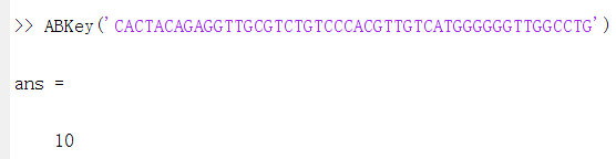
Figure 1: ANSWER
Simple flow chart of the "ABKey function"
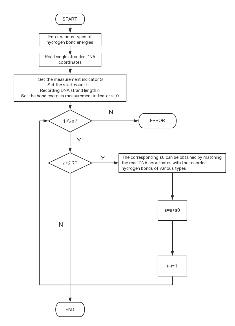
Figure 2: Chain length upper limit selection mechanism
Equation set of the ABKey function:
\begin{equation*} \begin{cases} \triangle G^{\circ}=\Sigma_{i} \triangle G_{i}^{\circ}\\ \triangle G^{\circ}=- RT\ln K^{\circ}\\ K_{d}=\frac{1}{K^{\circ}}\\ K_{d}\geq \widetilde{K_{d}}=28.8\times10^{-9}mol/L \end{cases} \end{equation*}
In fact, the number 10 happens to be a critical value. From 10 bases down, 9 or 8 base complements can also cause "competition" to occur spontaneously in the forward direction, but the fewer the complementary bases, the less likely it is that the aptamer - "complementary strand" double chain structure can be formed, resulting in the loss of the basis of "competition".
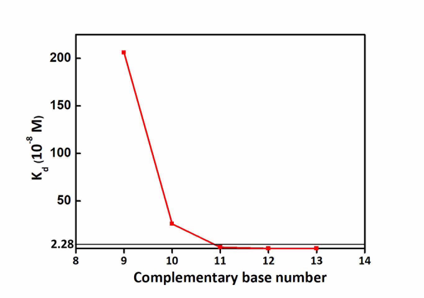
Figure 3: Line Chart
On the other hand, the minimum complementary value was set as 5 according to the literature.
References
[1] JOHN SANTALUCIA, JR*, A unified view of polymer, dumbbell, and oligonucleotide DNA nearest-neighbor thermodynamics, Proc Natl Acad Sci Anal Chem, 1998, 95, 1460-1465.
[2] Yanling Song, Zhi Zhu, Yuan An, Weiting Zhang, Huimin Zhang, Dan Liu, Chundong
Yu, Wei Duan, Chaoyong James Yang, Selection of DNA Aptamers against Epithelial Cell
Adhesion Molecule for Cancer Cell Imaging and Circulating Tumor Cell Capture, Proc Natl Acad Sci Anal Chem, 2013, 85, 4141-4149.
In order to ensure that the adaptor and the complementary sequence designed by us are not dissociated continuously under the impact of the liquid, which leads to false positive results, our modeling guides us to determine whether the designed rotation speed is reasonable.
Referring to the knowledge of chemical fluid flow and DNA structure, we designed a model that guided us to calculate the maximum rotational speed or maximum pressure difference under overall stability between the aptamer and complementary sequences. It's crucial to the hardware.
First, we focused on the relation between the flow velocity and rotation speed in the pipeline driven by centrifugal force only. Under the condition of laminar flow, we introduced several assumptions:
1. Ignoring the effects of gravity;
2. Ignoring the problem of force distribution in the vertical direction, and considered it as the uniform distribution;
3. As both ends of the fluid passed through the atmosphere, the pressure difference between the two ends of the fluid was ignored.
Based on the above hypothesis, the specific principle content and derivation are as follows:
The general formula of steady-state flow friction resistance of fluid in fluid mechanics is as follows:
\begin{equation} (p_{1}-p_{2})\pi r^{2}= \tau 2\pi rL \tag{2.1} \end{equation}
Then, in the same way as the settlement hypothesis, we introduced the fourth hypothesis: the fluid accelerates in the pipe for a short time, and the whole process is considered to be uniform.
According to the force analysis, when the fluid flows outward because of centrifugal, there is no pressure difference, and only the centripetal force is provided by the resistance, i.e.
\begin{equation} \tau 2\pi rL= F_{x} \tag{2.2} \end{equation}
At the same time, the flow velocity is usually reflected in the pressure drop, so we can combine (2.1) and (2.2), and relate the centripetal force $F_{x}$ to the pressure drop, and then show its effect on the flow rate. That is:
\begin{equation} (p_{1}-p_{2})\pi r^{2}= F_{x} \tag{2.3} \end{equation}
What's more,
\begin{equation} F_{x}=m\omega ^{2}R= 4\pi ^{2}mn^{2}R \tag{2.4} \end{equation}
\begin{equation} m= \rho \pi r^{2}L \tag{2.5} \end{equation}
From equations (2.3), (2.4) and (2.5), we can obtain the relation between pressure drop and flow velocity:
\begin{equation} \Delta p_{sf}=4\pi ^{2}n ^{2}\rho LR \tag{2.6} \end{equation} where $\tau$(Pa) represents the friction force, $\rho$(kg/m$^{3}$) represents the fluid density, n(r/s) represents the rotation speed, L(m) represents the fluid length, R(m) represents the length of fluid center to center of circle, r(m) represents radius of circular tube. For a variety of tubes, we can use different correction coefficients or hydraulic diameters to convert the tube diameter, but the tube shape is only reflected in r, and the r in the formula is also eliminated. Therefore, we considered equation (2.6) to be valid for any tube shape and theoretically free of error.
Then, because our fluid motion was carried out in the rectangular tube and is laminar flow, we can use the laminar flow relationship between pressure drop and flow velocity in the rectangular section pipe:
\begin{equation} \Delta p_{sf}=\frac{12\mu u_{b}L}{b^{2}}[1-\frac{192b}{\pi ^{5}a}th(\frac{\pi a}{2b})]^{-1} \tag{2.7} \end{equation}
By substituting equation (2.7) into equation (2.6), we obtained the laminar flow relationship between the speed and the flow velocity in the rectangular pipeline:
\begin{equation} u_{b}=\frac{4\pi ^{2}\rho b^{2}R}{12\mu}[1-\frac{192b}{\pi ^{5}a}th(\frac{\pi a}{2b})]\ast n^{2} \tag{2.8} \end{equation}
In the above, a(m) is the long side length of rectangular section pipeline and b(m) is the short side length.
At this point, we have completed the derivation of the first part about the relation between flow velocity and rotation speed.
The second part is to derive the relationship between drag force and flow velocity. Also under the condition of laminar flow, we introduced the following assumptions:
1.During the process, the fluid’s force on the solid is provided by the drag force;
2.No head loss is considered during liquid flow.
In the process of particle deposition, the drag equation is very consistent with the impact process of our fluid on DNA. The formula is as follows:
\begin{equation} F_{d}=\zeta A\frac{\rho u_{t}^{2}}{2} \tag{2.9} \end{equation}
In formula (2.9), $\zeta$ represents the drag coefficient with a dimension of 1; A(m$^{2}$) represents the movement of fluid's flowing through the plane area; $\rho$(kg/m$^{3}$) represents fluid density; $u_{t}$(m/s) represents the velocity of the particle relative to the fluid.
In laminar flow, the correlation between $\zeta$ and relative motion Reynolds number Ret and relative motion Reynolds number Ret is defined as:
\begin{equation} \zeta =\frac{24}{Re_{t}} \tag{2.10} \end{equation}
\begin{equation} Re_{t}=\frac{d_{s}u_{t}\rho }{\mu } \tag{2.11} \end{equation}
Substitute (2.10) and (2.11) into equation (2.9) and we have:
\begin{equation} F_{d}=\frac{12\mu u_{t}A}{d_{s}} \tag{2.12} \end{equation}
In equation (2.12), ds represents the diameter or equivalent diameter of particles. A is also related to ds. And because DNA is a double helix structure, the error in equivalent diameters is huge. Therefore, by simplifying the calculation of A, we want to keep A and get rid of ds.
There is Stokes Law in laminar flow:
\begin{equation} F_{d}=3\pi \mu u_{t}d_{s}\tag{2.13} \end{equation}
By combining equations (2.12) and (2.13), the final formula of traction can be obtained:
\begin{equation} F_{d}=\sqrt{36\pi A}\mu u_{t} \tag{2.14} \end{equation} where $\mu$ represents the viscosity of the fluid.
In addition, $u_{t}$ represents the velocity of the particle relative to the fluid. Since our adaptor is fixed on the plane, $u_{t}$=$u_{b}$(fluid velocity).
The third part is the dna-related model. To simplify the model, we introduced the following assumptions:
1.Simplified DNA molecular model, the flow through DNA as a rectangle, ignoring three- dimensional structure;
2.The simplified DNA model is supposed to be B-DNA and the base pair is WC pairing;
3.The base pair is considered to be completely dissociated after being destroyed by impact;
4.The forces between the stable DNA consider only the hydrogen bond between base pairs.
Following second part, we can use the DNA molecular structure to figure out the projected area A of the moving plane through which the fluid flows.
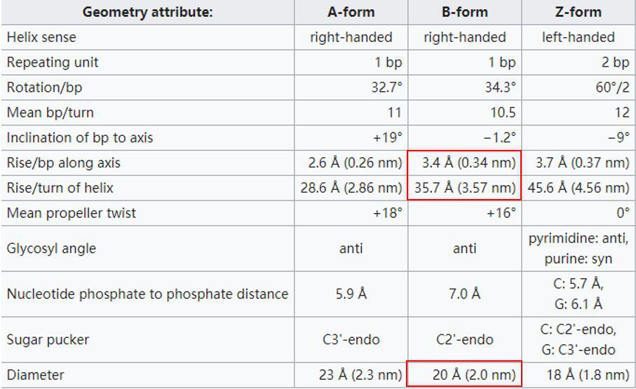
Figure 1: come from wiki [3]
We chose a most common B - DNA as a model. The distance that per chain of the double helix chains having a full circle around the axis (360$\eta$$^{\circ}$) up (or down) is 3.57 nm, usually containing 10.5 nucleotide. Therefore, each two adjacent base’s flat vertical distance is 0.34 nm. And the space between two chains are also certain, i.e., 2 nm.
Then, we have
\begin{equation} A= \frac{0.34\ast 10^{-9}\ast 2\ast 10^{-9}\ast n}{2} \tag{2.15} \end{equation}
In equation (2.15), A represents the area of the base pair through which the fluid flows, and n represents the nucleotide number used to activate crRNA. Because once the designed crRNA is determined, n is constant. So A is constant.
After finding the area A, we substitute it into equation (2.14), and the work of the total traction force can be obtained by the formula of force and work:
\begin{equation} W_{d}=F_{d}\ast \Delta x \tag{2.16} \end{equation}
Later, we obtained the following information in some literatures:
The two hydrogen bonds of the AT base pair basically break at the same time, and the three hydrogen bonds of the CG base pair break one by one. To prevent them from being swept away, what we need to consider is their energy barrier: the simultaneous breaking energy barrier of AT base pair is 23 KJ$\cdot$mol$^{-1}$, and CG base pair maximum energy barrier, namely the first hydrogen bond breaking threshold, is also 23 KJ$\cdot$mol$^{-1}$. So we can average out the base pairs at 23 KJ$\cdot$mol $^{-1}$ per base pair.
The distance between two hydrogen bonds that break AT base pairs is $\Delta$x$_{1}$=0.74-0.63=0.11nm; The distance to break the first hydrogen bond of the CG base is $\Delta$x$_{2}$= 0.72-0.65=0.07 nm.$^{[2]}$
We took the larger $\Delta$x as the fixed value of $\Delta$x, because the bigger the $\Delta$x gets, the more work it does.
Combining the three parts, we used the fluid dynamics model to guide our hardware design. At the same time, in order to ensure that there is no dissociation, we took the maximum energy barrier of a single base pair for conversion. Therefore, the rotation speed was independent from the complementary number.
We have simultaneous equations (2.8), (2.14), (2.15) and (2.16), and the final formula is:
\begin{equation} W_{d}=\frac{11}{300}\ast 10^{-18}\ast \sqrt{\frac{306\pi ^{5}k}{25}}\ast \rho b^{2}R\ast [1-\frac{192b}{\pi ^{5}a}th(\frac{\pi a}{2b})]\ast n^{2} \tag{2.17} \end{equation}
The above equation is substituted into the calculation equation
\begin{equation} W_{d}=\frac{11}{300}\ast 10^{-18}\ast \sqrt{\frac{306\pi ^{5}k}{25}}\ast \rho b^{2}R\ast [1-\frac{192b}{\pi ^{5}a}th(\frac{\pi a}{2b})]\ast n^{2}\leq \frac{23\ast 10^{3}}{6.022\ast 10^{23}} \tag{2.18} \end{equation} where k represents the number of nucleotides used to activate crRNA; $\rho$(kg/m $^ {3} $) represents fluid density, which is almost equal to the density of water; a(m) represents long side length of rectangular pipeline; b(m) represents short side length; R(m) represents the length from the fluid center to the center of the circle, which, in our hardware, is the length of the coating center to the center of the circle; n(r/s) represents rotation speed.
In our hardware design, a=b=1mm; k=21; $\rho$ is approximately equal to the density of water, which is 1000; and R is the length from the coating center to the center of the circle, which is 22.53mm. Substitute in the inequality and we get :n$\leq$19.70451801.
That is, the speed of n is not higher than 1182 r/min. Therefore, the rotor with the maximum speed of 500 r/min was selected by us considering the conditions of speed limitation, cost performance and portability.
Supplementary information on pressure drop as the driving force:
We used centrifugal force to be the driving force, while many teams used pumps instead. Taking this into consideration, and hoping that our model could be more complete, and we can help more people, we also provided the relevant derivation process and result formula of pressure drop.
In the first part, the relation between velocity of flow and speed of rotation is derived. After finding the relation between pressure drop and velocity of flow, we can establish the relation between flow velocity and the remaining two parts, and finallly obtain the formula.
In the rectangular section, the relationship between pressure drop and average flow velocity is:
\begin{equation} u_{b}=\frac{b^{2}\Delta p_{sf}}{12\mu L}[1-\frac{192b}{\pi ^{5}a}th(\frac{\pi a}{2b})] \tag{2.19} \end{equation}
By combining equations (2.17) with (2.14), (2.15) and (2.16), the final formula is:
\begin{equation} W_{d}=\frac{11}{1200}\ast 10^{-18}\ast \sqrt{\frac{306\pi k}{25}}\ast \frac{b^{2}}{L} \ast [1-\frac{192b}{\pi ^{5}a}th(\frac{\pi a}{2b})]\ast \Delta p_{sf} \tag{2.20} \end{equation}
The above equation can be substituted into the calculation, and the inequality is as follows:
\begin{equation} W_{d}=\frac{11}{1200}\ast 10^{-18}\ast \sqrt{\frac{306\pi k}{25}}\ast \frac{b^{2}}{L} \ast [1-\frac{192b}{\pi ^{5}a}th(\frac{\pi a}{2b})]\ast \Delta p_{sf}\leq \frac{23\ast 10^{3}}{6.022\ast 10^{23}} \tag{2.21} \end{equation} where k represents the number of nucleotides used to activate crRNA; L(m) represents the length of the fluid filling the pipe, which can be measured with a scale; a(m) represents long side length of rectangular pipeline; b(m) represents short side length; $\Delta p_{sf}$ (Pa) represents the pressure drop.
Analysis of model advantages and disadvantages:
1. The analysis of impact force is as follows:
First of all, to simplify the model, we simplified the DNA section to a rectangle, and in order not to introduce unknown factors into the comparison, we used the nucleotide number that activated crRNA to calculate, which would result in the model area larger than the actual area, resulting in the model impact force greater than the actual impact force;
We also omitted the friction force and other possible consumption and idealized all centrifugal forces (or pressure drops) into flow velocity for calculation, which would cause the model velocity to be greater than the actual flow velocity, and the model impact force to be greater than the actual impact force.
To sum up, we maximize all the items to maximize the possible impact.
2. The stability of base pair is analyzed as follows:
Our hypothesis is that the interaction force between base pairs is only provided by hydrogen bonds to maintain its stability. However, in practical cases, other intermolecular forces, such as van der Waals force and salt bond, may enhance the stability between base pairs, so the model stability is less than the actual stability.
Therefore, in the process of modeling, the impact force is idealized to the maximum. And the most stable energy barrier is also used for calculation on the premise that other forces of the stable structure are ignored. That is to say, the calculated critical speed or critical pressure strength should be the minimum and most conservative value, which is very credible.
Based on the above analysis, we have reasons to believe that our model is reasonable and feasible.
References
[1] Chai chengjing, Zhang guoliang. Chemical Fluid Flow And Heat Transfer(the second edition)[M], Beijing,Chemical Industry Press. 2007, 40-45$\&$129-132.
[2] SG WU, D FENG, Free Energy Calculation for Base Pair Dissociation in a DNA Duplex. Acta Physico-Chimica Sinica. 2016, 32 (5), 1282-1288
[3] https://en.wikipedia.org/wiki/A-DNA
1、Protein model
STEP1: The target sequence of human epithelial adhesion molecules was found at NCBI's GenBank: AAH14785.1$^{[1]-[2]}$
STEP2: Swiss-model was used for protein modeling prediction.
The Protein model predicted as follows: $^{[3]-[7]}$
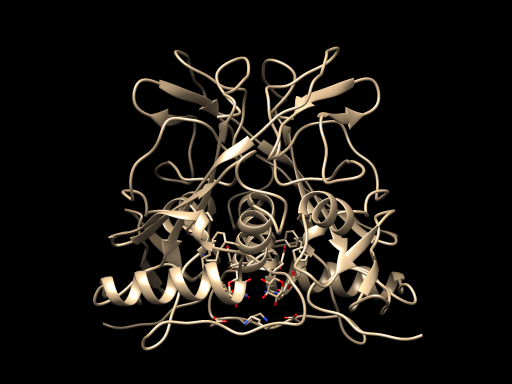
2、DNA molecule model
When we were worried about the establishment of secondary three-dimensional structure of DNA, a literature about establishing ssDNA model through RNA model gave us a new inspiration.$^{[8]}$
STEP1: We predicted the secondary two-dimensional structure of ssDNA in DNA - Folding - Form$^{[9]}$ by using the structure reported in the original literature: "....(((((.......))))) ((((........)))).((....))..".$^{[10]}$
The conditions are as follows:
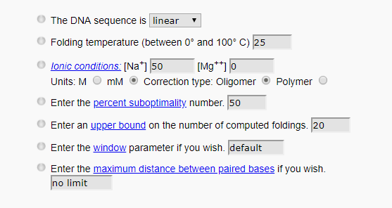
The predicted results are as follows:
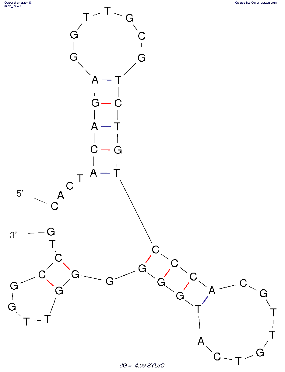
STEP2: We tried another method of RNA modeling in literature$^{[11]}$, and finally succeeded in establishing our RNA model in 3dRNA.$^{[12]-[14]}$
The RNA model is shown below:
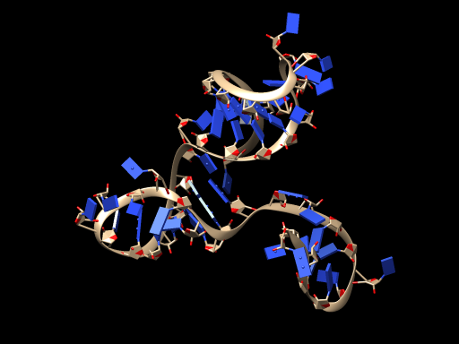
STEP3: We successfully transformed the RNA model into ssDNA model on VMD.$^{[15]}$
The DNA model is shown below:
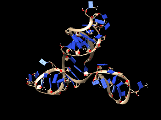
3、Molecular docking model
Finally, we made molecular docking between ssDNA model and protein model using Escher NG in VEGA ZZ.$^{[16]}$
The results of the docking model are as follows:
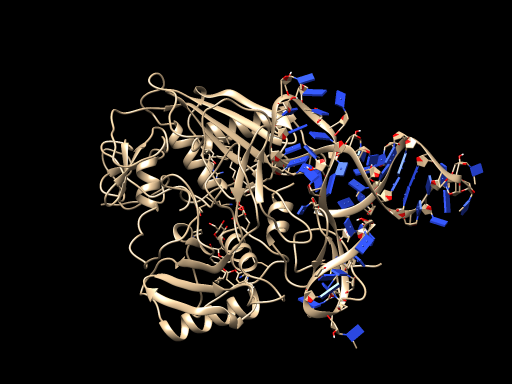
In addition, we used UCSF Chimera to output our modeling figures for each step.$^{[17]}$
References
[1] MGCP Team. Generation and initial analysis of more than 15,000 full-length human and mouse cDNA sequences. Proc. Natl. Acad. Sci. U.S.A., 2002.99 (26), 16899-16903.
[2] NIH MGC Project. Direct Submission. Submitted (01-OCT-2001) National Institutes of
Health, Mammalian Gene Collection (MGC), Bethesda, MD 20892-2590, USA.
[3] Waterhouse, A., Bertoni, M., Bienert, S., Studer, G., Tauriello, G., Gumienny, R., Heer, F.T., de Beer, T.A.P., Rempfer, C., Bordoli, L., Lepore, R., Schwede, T. SWISS-MODEL: 3 homology modelling of protein structures and complexes. Nucleic Acids Res. 2018.46(W1), W296-W303.
[4] Bienert, S., Waterhouse, A., de Beer, T.A.P., Tauriello, G., Studer, G., Bordoli, L., Schwede, T. The SWISS-MODEL Repository - new features and functionality. Nucleic Acids Res. 2017. 45, D313-D319.
[5] Guex, N., Peitsch, M.C., Schwede, T. Automated comparative protein structure modeling with SWISS-MODEL and Swiss-PdbViewer: A historical perspective. Electrophoresis 30, 2009. S162-S173.
[6] Benkert, P., Biasini, M., Schwede, T. Toward the estimation of the absolute quality of individual protein structure models. Bioinformatics 27, 2011. 343-350.
[7] Bertoni, M., Kiefer, F., Biasini, M., Bordoli, L., Schwede, T. Modeling protein quaternary structure of homo- and hetero-oligomers beyond binary interactions by homology. Scientific Reports 7 , 2017.
[8] Jeddi I, Saiz L. Three-dimensional modeling of single stranded DNA hairpins for aptamer-
based biosensors. Scientific Reports, 2017 , 7 (1) :1178.
[9] M Zuker. Mfold web server for nucleic acid folding and hybridization prediction. Nucleic
acids research, 2003 Jul 1;31(13):3406-15.
[10] Yanling Song, Zhi Zhu, Yuan An, Weiting Zhang, Huimin Zhang, Dan Liu, Chundong
Yu, Wei Duan, Chaoyong James Yang, Selection of DNA Aptamers against Epithelial Cell
Adhesion Molecule for Cancer Cell Imaging and Circulating Tumor Cell Capture, Anal
Chem, 2013, 85, 4141-4149.
[11] D Antunes, NAN Jorge, ER Caffarena, F Passetti. Using RNA Sequence and Structure for
the Prediction of Riboswitch Aptamer: A Comprehensive Review of Available Software
and Tools. Frontiers in Genetics, 2017, 8 :231.
[12] Zhao, Y., et al., Automated and fast building of three-dimensional RNA structures. Scientific Reports, 2012. 2: p. 734.
[13] Wang, J., et al., Optimization of RNA 3D structure prediction using evolutionary restraints of nucleotide-nucleotide interactions from direct coupling analysis. Nucleic Acids Res. 2017,
45 (11).
[14] Wang, J., et al., 3dRNAscore: a distance and torsion angle dependent evaluation function
of 3D RNA structures. Nucleic Acids Res, 2015. 43(10): p. e63.
[15] https://www.ks.uiuc.edu/Research/vmd/vmd-1.9.3/winrelnotes.html
[16] http://www.vegazz.net/
[17] http://www.rbvi.ucsf.edu/chimera
Derivation of rate equation of the competitive reaction:
$$AC+P\rightleftharpoons AP+C \qquad K=\frac{k_{1}}{k_{-1}}$$ where A represents an aptamer, C represents a "complementary strand" of the aptamer, P represents the target protein of the aptamer, AC represents an aptamer-"complementary strand" complex, and AP represents an aptamer-protein complex; K is the equilibrium constant of the competitive reaction, k$_{1}$ is the reaction rate constant of the forward reaction, k$_{-1}$ is the rate constant of the reverse reaction.
It is assumed that both the forward reaction and the reverse reaction are mixed secondary reactions$^{[1]}$, then the expression of reaction rate can be written down:
\begin{equation} r=\frac{d[C]}{dt}=k_{1}[AC][P]-k_{-1}[AP][C] \tag{4.1} \end{equation}
For the reaction system, there are material relationships:
\begin{equation} [A]_{0}=[A]+[AC]+[AP] \tag{4.2} \end{equation} \begin{equation} [C]_{0}=[C]+[AC] \tag{4.3} \end{equation} \begin{equation} [P]_{0}=[P]+[AP] \tag{4.4} \end{equation} where [A]$_{0}$ is the total concentration of the A-related species in the reaction system, [C]$_{0}$ is the total concentration of the C-related species in the reaction system; [A] is the concentration of the "free" aptamer. In fact, the body of the aptamer is immobilized on a solid phase and does not escape into the solution. Here, the concentration of the aptamer that binds to neither the target protein nor the "complementary strand" is indicated by [A]. Obviously, the concentration of the "free" aptamer in the reaction system is very low and can be ignored, so equation (4.2) can be written as:
\begin{equation} [A]_{0}=[AC]+[AP]\tag{4.5} \end{equation}
We believe that the aptamer and the "complementary strand" are combined in a 1:1 ratio at the start of the reaction, i.e.
\begin{equation} [A]_{0}=[C]_{0}\tag{4.6} \end{equation}
It can be written out from equation (4.3)(4.5)(4.6):
\begin{equation} [C]=[AP]\tag{4.7} \end{equation}
Therefore, the expression of the reaction rate can be written as:
\begin{equation} \frac{d[C]}{dt}=k_{1}([A]_{0}-[AP])([P]_{0}-[AP])-k_{-1}[AP][C]\tag{4.8} \end{equation}
Substituting (4.7) into (4.8) gives:
\begin{equation} \frac{d[C]}{dt}=k_{1}([A]_{0}-[C])([P]_{0}-[C])-k_{-1}[C]^{2}\tag{4.9} \end{equation}
i.e.\begin{equation} \frac{d[C]}{dt}=(k_{1}-k_{-1})[C]^{2}-k_{1}([A]_{0}-[P]_{0})[C]+k_{1}[A]_{0}[P]_{0}\tag{4.10} \end{equation}
This is the differential form of the competitive reaction rate equation. Since both [A]$_{0}$ and [P]$_{0}$ are known at the time of verification; at a certain temperature, the values of k$_{1}$ and k$_{-1}$ are also fixed for the determined reaction. Therefore, for the shifting and integration of (4.10), we can get:
\begin{equation} \int_{0}^{t}dt=\int_{[C]_{0}}^{[C]}\frac{d[C]}{a[C]^{2}+b[C]+c}\tag{4.11} \end{equation} where a=k$_{1}$-k$_{-1}$, b=-k$_{-1}$([A]$_{0}$+[P]$_{0}$), c=k$_{1}$[A]$_{0}$[P]$_{0}$.
It's worth noting that\begin{eqnarray} b^{2}-4ac&=&k_{1}^{2}([A]_{0}+[P]_{0})^{2}-4(k_{1}-k_{-1})k_{1}[A]_{0}[P]_{0}\\&=&k_{1}^{2}([A]_{0}^{2}+[P]_{0}^{2}+2[A]_{0}[P]_{0})-4(k_{1}-k_{-1})k_{1}[A]_{0}[P]_{0}\\&=&k_{1}^{2}([A]_{0}^{2}+[P]_{0}^{2})+[2k_{1}^{2}-4(k_{1}-k_{-1})k_{1}][A]_{0}[P]_{0}\\&=&k_{1}^{2}([A]_{0}^{2}+[P]_{0}^{2})-2k_{1}^{2}[A]_{0}[P]_{0}+4k_{1}k_{-1}[A]_{0}[P]_{0}\\&\geq&0+4k_{1}k_{-1}[A]_{0}[P]_{0}\\&>&0 \end{eqnarray}
Therefore, the integral form of the competitive reaction rate equation is \begin{equation} t=\frac{1}{x_{2}-x_{1}}\ln(\frac{\sqrt{a}[C]+x_{1}}{\sqrt{a}[C]+x_{2}})\mid_{[C]_{0}}^{[C]}\tag{4.12} \end{equation} Where x$_{1}$ and x$_{2}$ are two roots of the equation $x^{2}-\frac{b}{\sqrt{a}}x+c=0$.
EXPERIMENT: Experiments were performed using the optimized "complementary strand" sequence. The 3' end of the "complementary strand" carries the FAM tag. At a certain temperature, [A]$_ {0} $ and [P]$_ {0} $ were fixed, and [C]$_{0}$ of all experimental groups was set to be the same, so that the single variable of the experiment was the time t of the reaction. The aptamer and its "complementary strand" are immobilized on the magnetic beads. After the protein is added, the magnetic beads are sucked to the bottom by the magnet immediately after the reaction for different time, and the supernatant is taken to detect the fluorescence intensity. By making a t-I figure, since the fluorescence intensity I is proportional to the concentration [C]$^{[2]}$, the form of the relation between t and I is compared with (4.12) to verify whether the derivation of the rate equation is correct or not.
References
[1] Sun shigang, etc. Pysical Chemistry (the second edition), Xiamen: Xiamen University Press, 2013, 13-33.
[2] Xu jingou, Wang zhunben, etc. Fluorescence Analysis (the third edition), Beijing: Science Press, 2006, 12-13.

- Home
- Basic Part
- About us
- Composite Part
- Attribution
- Design
- Modeling
- Engagemen
- Biosafety
- Contribution
- Collaboration
- Protocols
- Notebook
- Description
- Experiment