Team:BNDS CHINA/Model
Our model helped us to optimize the A. hydrophila sensor devices. At first,
we measured the concentration of C4-HSL in A.
hydrophila culture by using mass spectrum. Then, we tested the GFP
production rate of sensor device I. The experimental results were characterized
by using Hill equation, which modelled the GFP synthesis rate as a function of
input concentration of the inducer, C4-HSL. However, when we predicted the
efficiency of this device in real environment by the derived function, we found
the fluorescence was too low to be detected. Therefore, we adjusted our design
by increasing rhlR RBS strength and modelled the experimental results by using
Hill equation again. This time, we found the device’s (BBa_K2548001) fluorescence
in real environment was enough to be detected. More importantly, our model can
help to indicate the A. hydrophila
concentration in different environments, and alerts the aquaculture managers
the danger of pathogen infection. In addition, we visualize the data in
three-dimensions to show how GFP production rate per cell over time at different C4-HSL inducer
concentrations to characterize the sensor in a more comprehensive way. In order to characterize the expression system, we first acquired the experiment data of
GFP production rate per cell (RFU per Abs per min) under different
concentration of inducers In biochemistry, the binding ability
of a ligand to a macromolecule is often increased if other ligands have already
present on the same macromolecule. The hill equation is used to determine the cooperativeness
of a ligand binding to its receptor, and it can describe the relationship
between the expression level of genes which are regulated and the quantity of
regulatory factors. We model the GFP synthesis rate
( The figure above shows the modeling result of Device I. The derived equation is: And the correlation coefficient of the equation is 0.9816. The figure above shows the modelling result of Device II. The derived equation is: And the correlation coefficient of the equation is 0.9897. The figure above shows the modeling result of Device III. The derived equation is: And the correlation coefficient of the equation is 0.9952. We used the two equations to predict the efficiency of the sensor devices. See the analysis of
these results at demonstrate. The GFP production rate is converted as RFU per Abs per min,
calculated through the arithmetic average of three trails to eliminate the
systematic and experimental errors. The three axes are named respectively as
Time (min),
Time( t ) ∈ [ 0,220 ] with interval of 10mins . C4-HSL concentration ( M ) ∈ [
GFP production rate ∈ [ 0,4 ] from experimental test experience. The modeling is achieved through Mathematica 11. All discrete
points are contained in manual data set. To show the variation tendency of
data, we took MeshFunction to connect the adjacent
points and present the regional changing trend, like the concavity or
convexity. To specify and highlight the progressive changes of GFP production
rate, we took the PlotLegends Function of Colorful
pattern. The three-dimension graph can be rotated 360 degrees and observed from
different views. To illustrate the three-dimensional data in plane and the
height ( z -axis value) is represented through the
shade of color. The image is generated through ListDensityPlot
Function. Saeidi, N., Wong, C. K., Lo, T., Nguyen, H. X., Ling, H.,
Leong, S. S., . . . Chang, M. W. (2014). Engineering
microbes to sense and eradicate Pseudomonas aeruginosa, a human pathogen. Molecular Systems Biology, 7(1),
521-521. doi:10.1038/msb.2011.55Model
I. Summary
II. Assumptions
III. Design of Characterizations
 (M) (see experiment). Then the experimental
data were fitted using the Hill equation:
(M) (see experiment). Then the experimental
data were fitted using the Hill equation:
 ) as a function of input concentration of
(
) as a function of input concentration of
( ). The four parameters
(
). The four parameters
( ,
,
 ,
,
 ,
,
 ) were estimated to obtain the best fit curve by performing a
non-linear curve fitting using the experimental data. Among the parameters, n
is the Hill coefficient, which describes the cooperativity; C is the
concentration of C4-HSL (M) which produces half occupation. This curve fitting was performed using Logger Pro. (Saeidi et
al, 2011).
) were estimated to obtain the best fit curve by performing a
non-linear curve fitting using the experimental data. Among the parameters, n
is the Hill coefficient, which describes the cooperativity; C is the
concentration of C4-HSL (M) which produces half occupation. This curve fitting was performed using Logger Pro. (Saeidi et
al, 2011).IV. Results of Characterizations of Sensor Device I and Device II
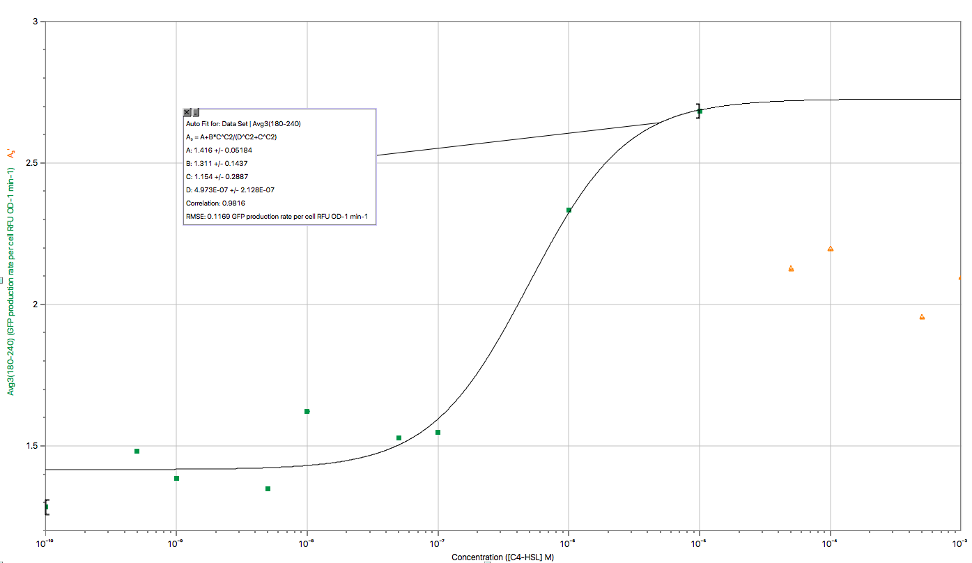
Fig 1. Characterization of Sensor Device I (BBa_K2548000 + BBa_K2548003)
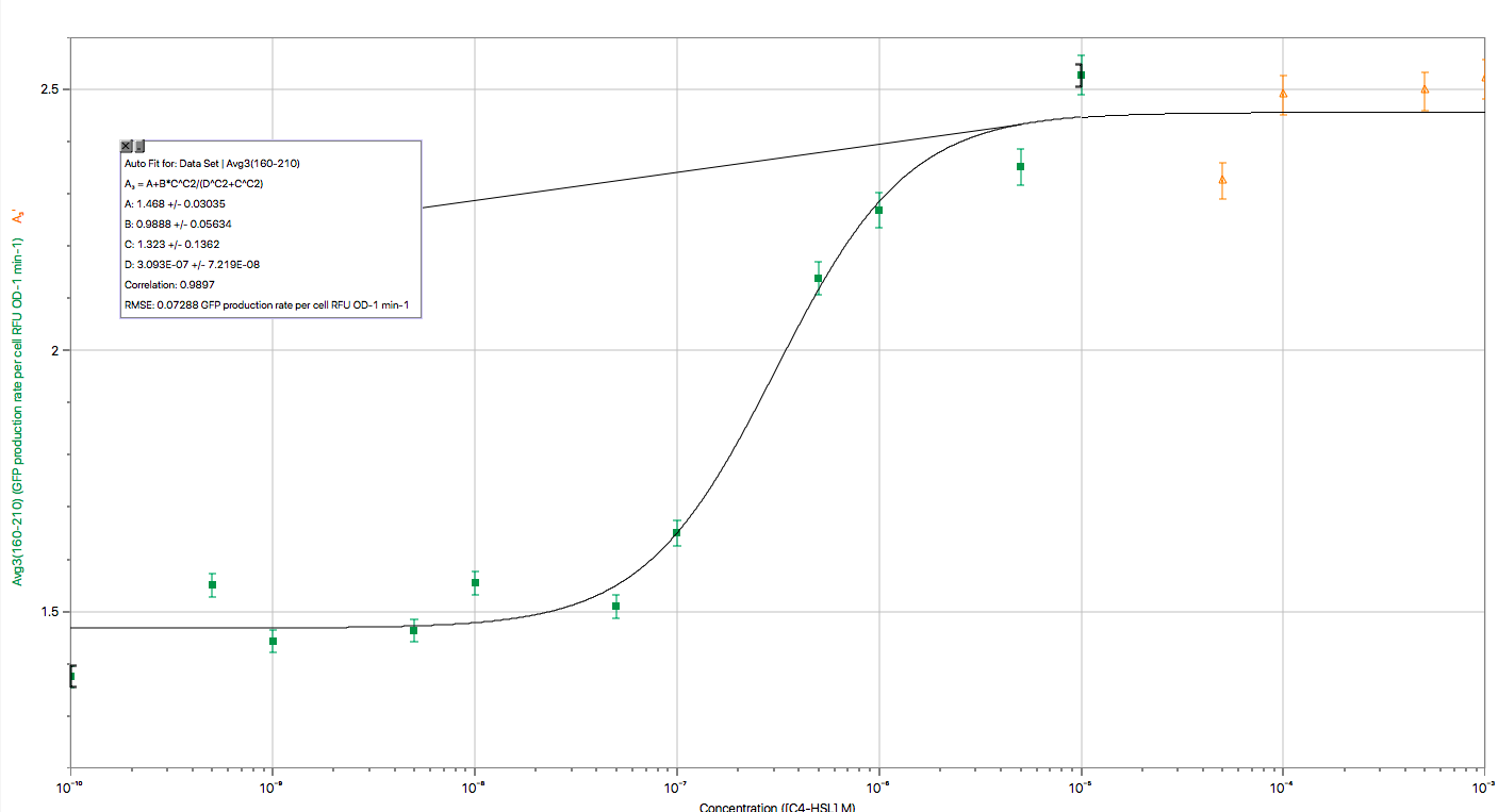
Fig 2. Characterization of Sensor Device II
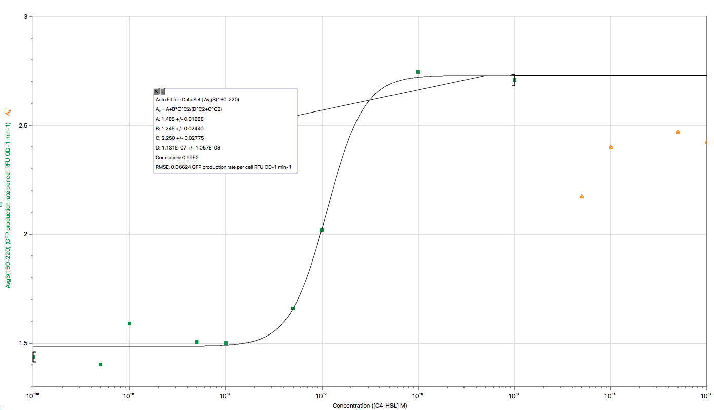
Fig 3. Characterization of Sensor Device II (BBa_K2548001 + BBa_K2548003)
V. Visualization of Data in Three-Dimensions
 , and GFP
production rate. The three variables are defined respectively in different
sets, automatically imported from Excel to maintain the efficiency and
productivity of modeling.
, and GFP
production rate. The three variables are defined respectively in different
sets, automatically imported from Excel to maintain the efficiency and
productivity of modeling.  ,
,
 ] for geometric
sequence of ratio of 5 . To maintain the integrity of image, the value of
concentration is replaced by marks from 1-15.
] for geometric
sequence of ratio of 5 . To maintain the integrity of image, the value of
concentration is replaced by marks from 1-15. 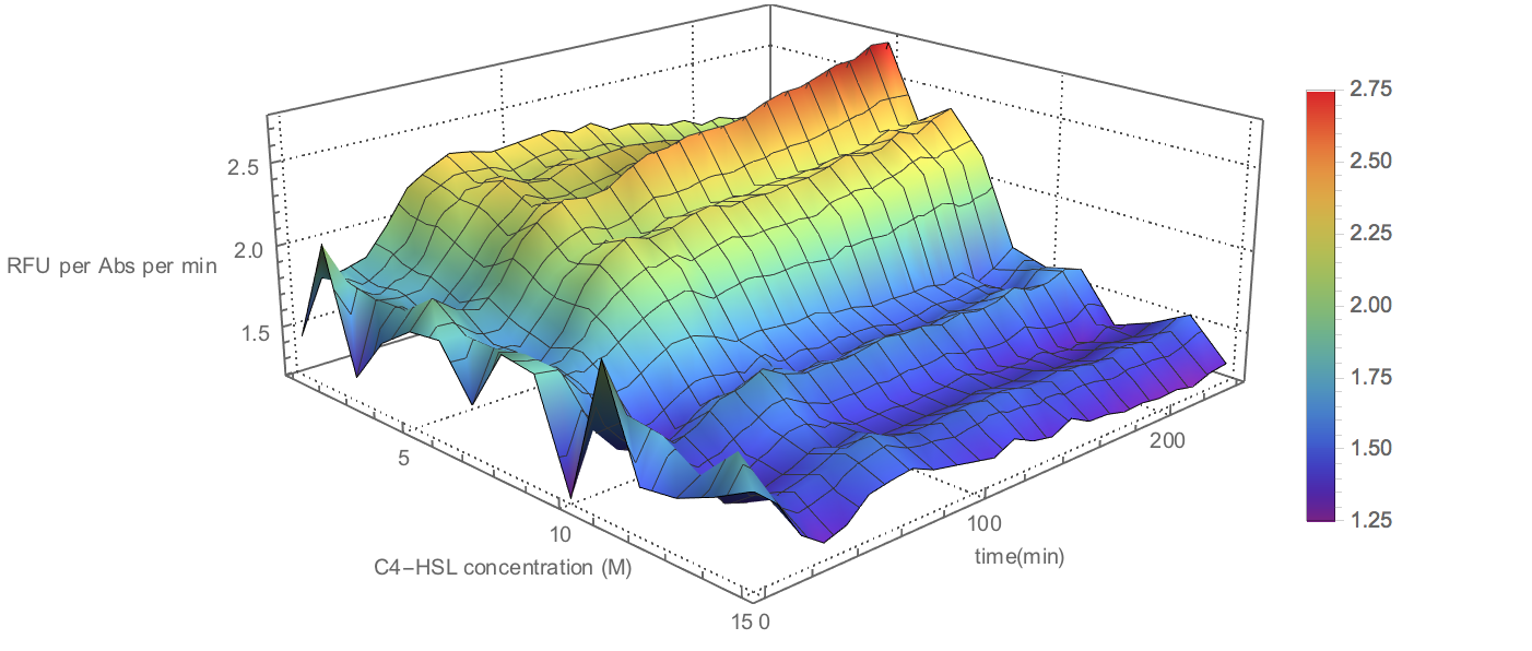
Fig 4. Visualization of Sensor Device I Experiment Data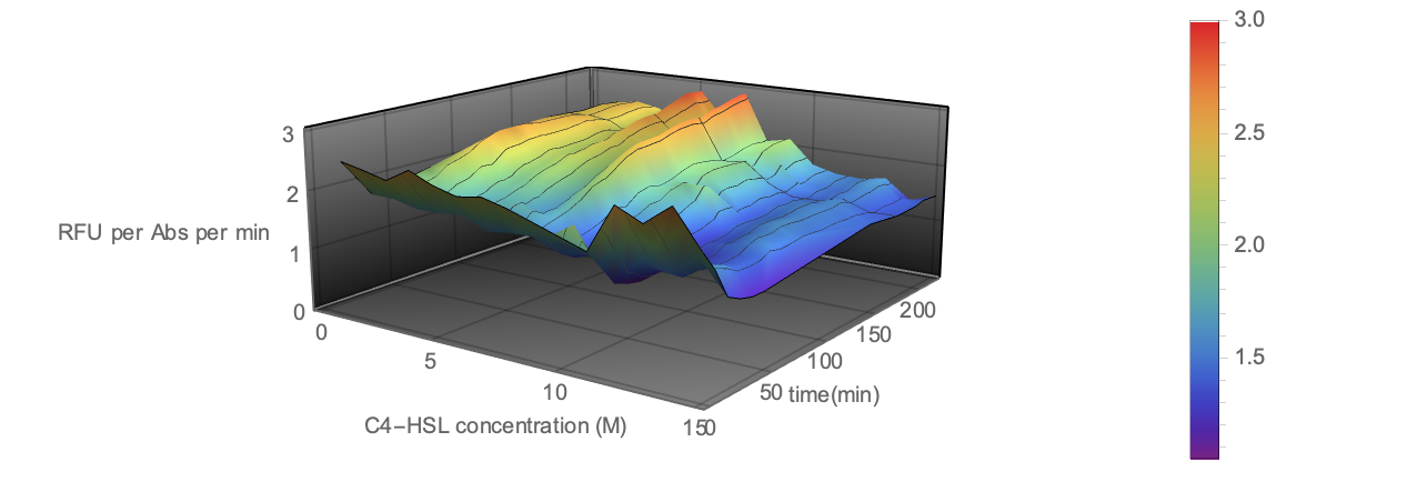
Fig 5. Visualization of Sensor Device III Experiment Data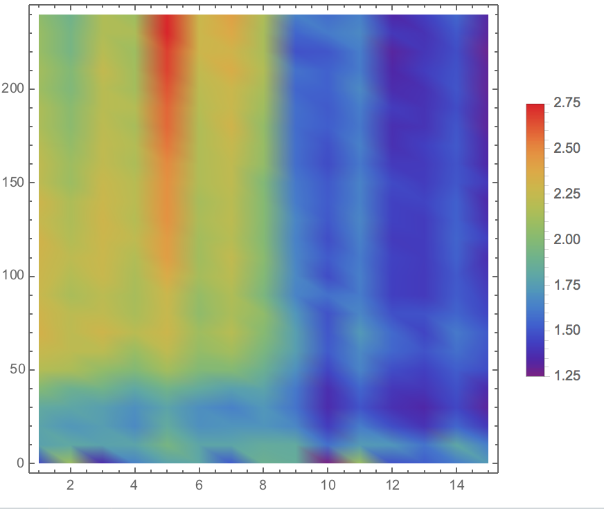
Fig 6. Visualization of Sensor Device I Experiment Data in Plane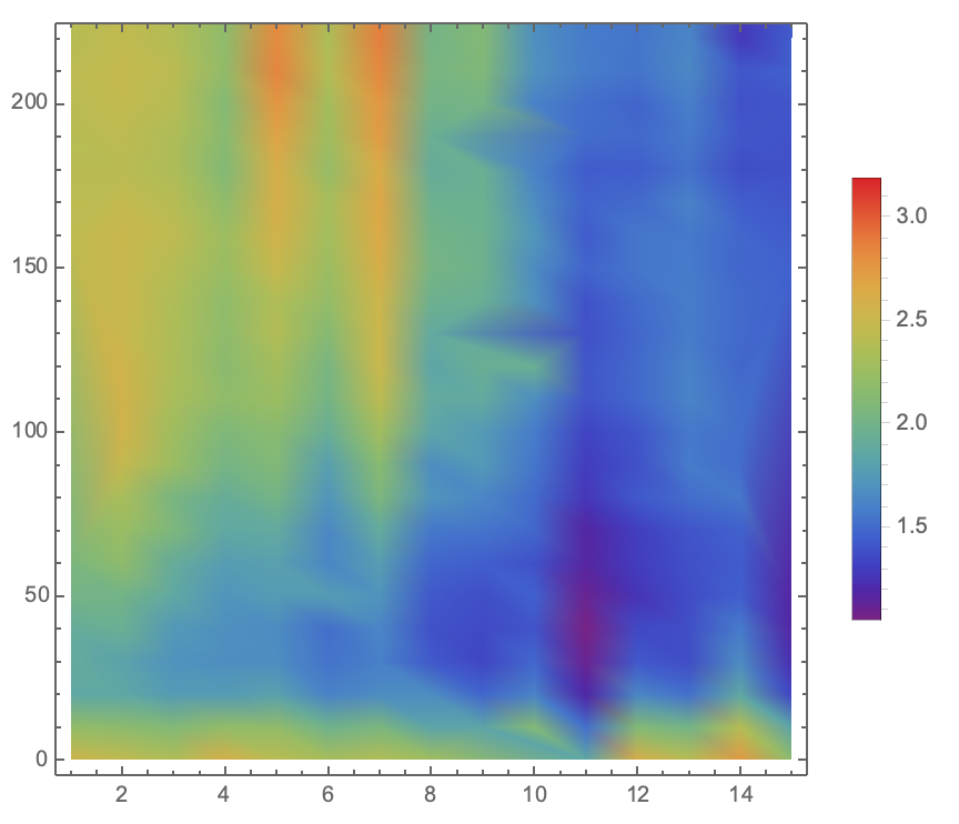
Fig 7. Visualization of Sensor Device III Experiment Data in PlaneReferences