Team:TU Darmstadt/Model

Modeling

Abstract

For this year's project, we wanted to predict the composition of our polymer. This is very important for our project, because the reaction of our different monomers during the polymerization influences properties like the crystallinity of the polymer, and through that also our application approach.
For medical applications it is necessary to have a defined composition, and thereby specific properties of the used polymer, for example to prevent inflammatory reactions.

During our Human Practices work, we entered in a conversation with Evonik Industries, a company focused on the production of speciality chemicals. Talking to them was part of our concept to reach out to specialists to discuss our project idea.
Our talk centered around the production of PLGA. Eventually, we came to talk about the probability of our different monomers in reaction with each other and they explained that glycolic acid will incorporate better into our polymer than lactic acid.
As this could lead to different properties of the polymer, because of the possible formation of blocks of glycolic acid during the polymerization, we decided to develop a kinetic model of our polymerization process ourselves. Evonik's input was greatly appreciated and sparked the idea for our modeling approach. For more information on how they influenced our project in other ways, visit the Human Practices page.

Using the kinetic model, we were aiming to obtain information regarding the monomer composition of our different generated polymers, and thereby enable the prediction of their properties.

Introduction

Due to our project, we focused on the mechanism of polymerization of different monomers into a co‑polymer.
Co‑polymers in general consist of more than one type of monomer. They have to be distinguished in bipolymers, consisting of two different monomers, and terpolymers, consisting of three different monomers. For our modeling approach, we focused on the polymerization of two different monomers (glycolic acid and lactic acid). The resulting co‑polymer was PLGA.
Different co‑polymers can be defined, depending on the sequence of the monomers. The first possibility is a more or less random sequence of the monomers, which leads to a statistical co‑polymer. The second possibility is a completely alternating copolymer, and the third possibility is a block polymer in which the monomers form blocks of only one kind of monomer.
Different polymerization mechanisms facilitate different polymerization patterns, but are not a direct information on the pattern. Radical polymerization tends to yield statistical alternating polymers, while ionic polymerization methods often lead to block polymerization.
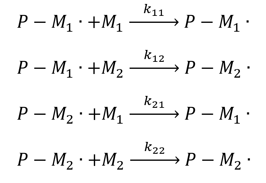
As soon as the polymerization is not 100 % complete and all monomers are depleted, the co‑polymer composition is not equal to the monomer composition chosen at the reaction start. This is due to four different possible elongation steps, depending on the last (active) monomer (M_i) in the growing chain P, as well as the next monomer that is added.

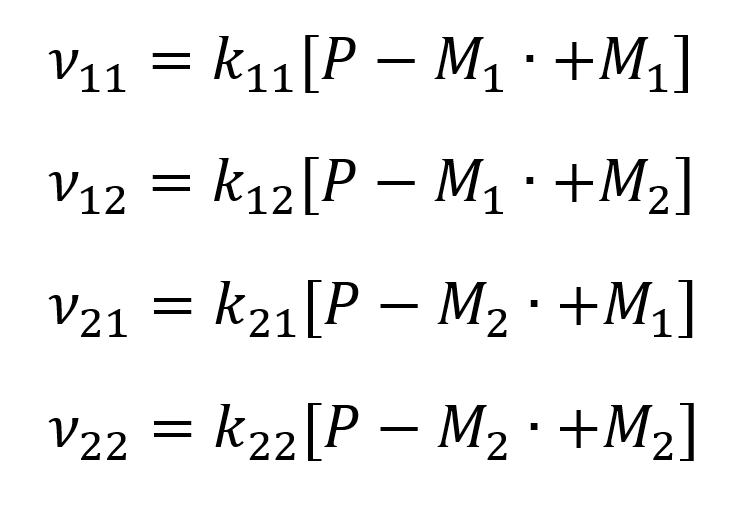
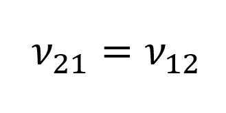
Because only the last monomer of the polymer chain is considered for elongation reactivity, the reaction follows Markov statistics of first order, which leads to the following reaction velocities ν:

Actually, the used method is only valid for radical polymerization. For anionic polymerization, the initiator would be needed to be considered for exact calculations of the expected yield, but in approximation, these simplified calculations can be used as well.
The above-mentioned different co‑polymerization patterns depend on the different affinities of the active end- chain monomer of the polymer to the two different free monomers.
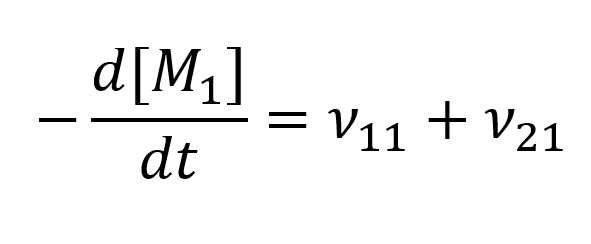
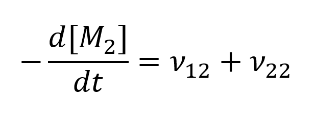
When the preferred monomers deplete, the less-favored monomer is incorporated into the polymer chain. The extreme example of this difference is a two-block co‑polymer, where the two different monomers separate during polymerization, as first one monomer is incorporated completely, and then the other. For the calculations, the rate of reaction for the two monomers is needed and can be described, with M₁ and M₂ being the respective monomers 1 and 2, as:

For our calculations of the kinetic model, due to the huge chain length, the depletion of monomers during initiation can be ignored, and only the depletion of monomers during elongation is taken into account. Furthermore, because we have a living polymer, no termination is observed, and thus can’t be calculated. These assumptions lead to the following equation for the relation of the depletion of the two monomers:

For the active sites, quasi-stationary properties can be assumed:

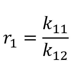
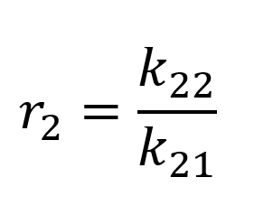
For a better understanding which co‑polymers are formed, co‑polymerization parameters r_i are introduced. The co‑polymerization parameters r₁ and r₂ show the preference of the monomer addition on the active monomer site of the polymer chain:

The r-values are characteristic for different monomer-pairs and their relation to each other dictates the co‑polymer composition. For example:
• r₁=r₂=1 leads to k₁₁=k₁₂ and k₂₁=k₂₂ describe an ideal co‑polymerization for an absolute stochastic co‑polymer
• r₁>1, r₂<1 leads to k₁₁>k₁₂ and k₂₁>k₂₂ describe a statistical co‑polymer where one monomer shows longer chains than the other
• r₁>1, r₂>1 leads to k₁₁>k₁₂ and k₂₁<k₂₂ describe the preference of the incorporation of the same monomers, that leads to the formation of block-polymers.
• r₁=r₂=∞ describes the homopolymerization and only a polymer mixture is obtained
• r₁<1, r₂<1 leads to k₁₁<k₁₂ and k₂₁>k₂₂ describes the incorporation preference of the other monomer over the same monomer, which leads to an alternating polymer
The co‑polymerization parameters can be calculated when the starting composition of the monomer mixture and the end composition of the co‑polymer in molar ratios is known, using the Kelen‑Tuedos‑equation, which can be used until 50 % polymer yield.

Implementation

The basis for our calculations is the Kelen‑Tuedos‑equation shown below, which introduces a few parameters.

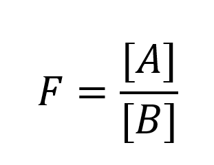
F is the fraction of used monomer composition at the start of the reaction, with A being the molar ratio of monomer 1 and B being the molar ratio of monomer 2.

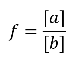
f is the fraction of monomer composition in the final co‑polymer after the reaction, with a being the molar ratio of monomer 1 and b being the molar ratio of monomer 2.

When f and F are known or calculated, the helping variable α of the Kelen‑Tuedos‑equation can be obtained as follows:

The more datapoints for H are calculated, the more exact the approximation of Kelen and Tuedos becomes.
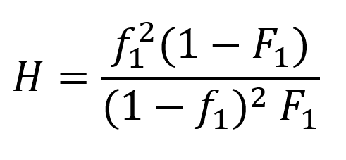
To calculate at least two H‑values, two sets of datapoints of applied monomer composition and achieved monomer composition are inserted into the following formula:

With the calculated values for α and the datapoints, a linear equation system with the Kelen‑Tuedos‑equation can be obtained, and thus the co‑polymerization parameters can be calculated. After the r‑values are calculated as well as α, the monomer composition of the polymer with a given start ratio F can be calculated with the changed Kelen‑Tuedos‑equation:

Results

For the calculations of the desired values, two pairs of data points are considered. The used values are from two reaction mixtures and the data of the f‑values come from NMR analysis of the molar ratio of the two monomers in the polymer. In our case A/a stands for lactide, and B/b for glycolide, with the majuscule indicating the starting molar ratio, and the minuscule the ratio after the reaction.

The used data points are shown in table 1.

Table 1: Ratios of molar monomer composition in % at the beginning of the reaction (F) or incorporated into the polymer (f) for two different reaction mixtures.

	reaction 1	reaction 2
F	75/25	2/3 / 1/3
f	59.13/40.87	38.76/61.24

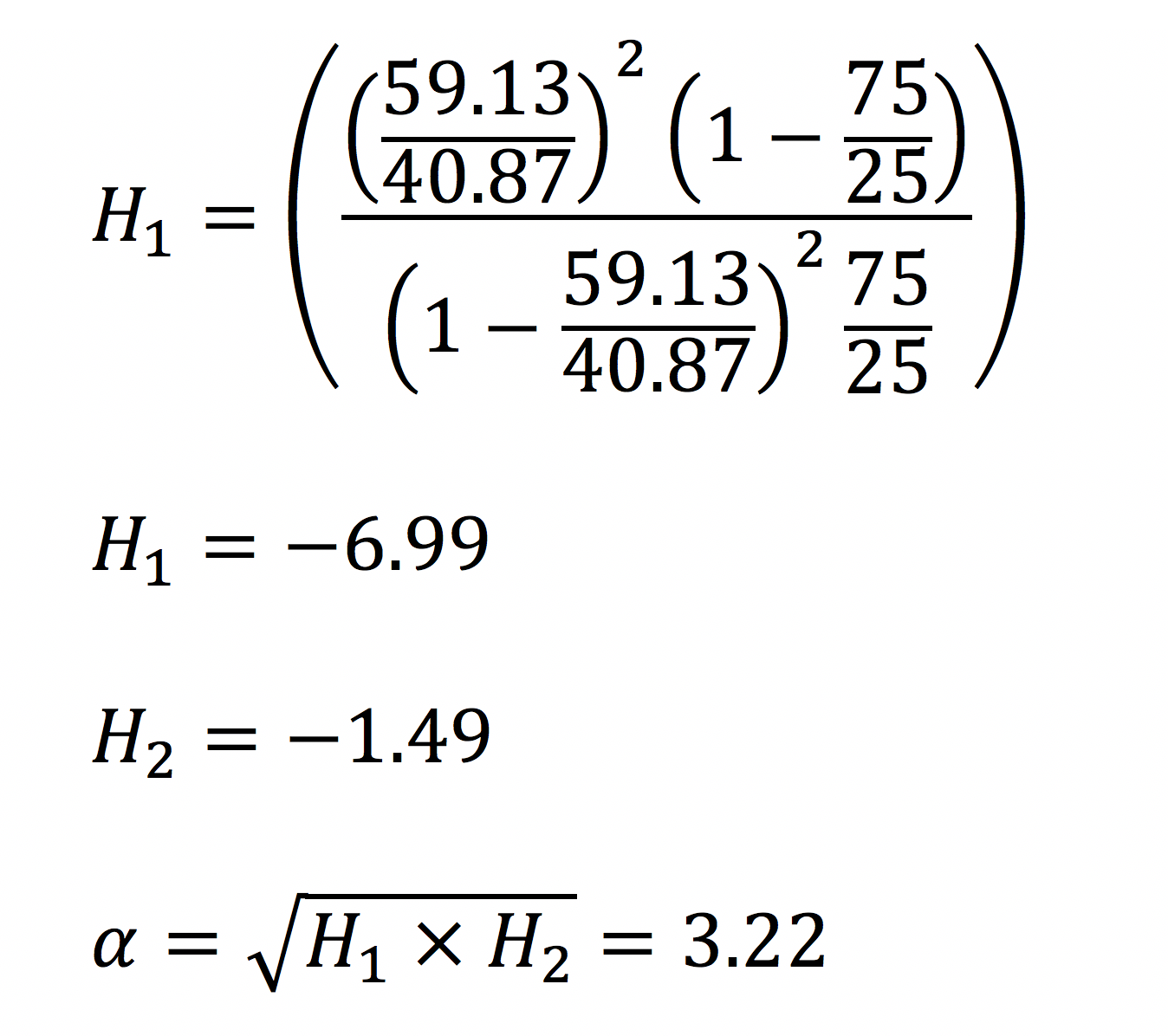
From the experimental data, the values for H can be calculated.

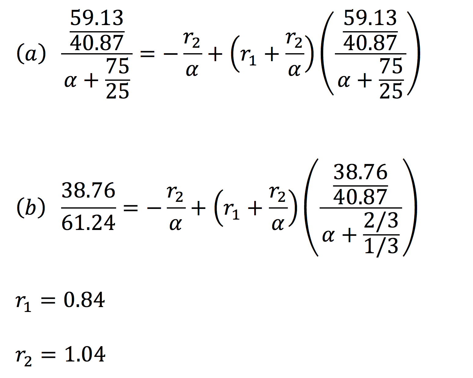
When different H‑ values are known, the helping variable α can be calculated and incorporated into the Kelen‑Tuedos‑equation. In combination with the experimental data points, a system of linear equations is made to calculate r₁ and r₂ as follows:

Now that the two needed copolymerization parameters are known, the final composition of monomers in a polymer can be calculated with the equation:

In the following table different theoretical monomer compositions in correlation to the used starting monomer composition are listed as calculated.

Table 2: Relative monomer composition f in dependence of the initial monomer composition in the reaction mixture F calculated after Kelen and Tuedos using the obtained values for α, r₁ and r₂

F	1.5	2	2.5	3	3.5	4	4.5	5
f	0.22	0.64	1.06	1.48	1.90	2.32	2.74	3.16

The calculated data is an approximation considered valid, if the yield of polymer is smaller than 50 %, and if F is bigger than 1.25.

Conclusion

The calculated r‑values with r₁=0.84 and r₂=1.04 show that glycolide is slightly better incorporated into the polymer than lactide. In this way we were able to prove the recommendation of Evonik.
This yields a stochastic alternating copolymer with more glycolide in the final polymer than lactide, at least for the observed conversion rates of about 20 % polymer production. When the polymer yield increases further and rises towards 100 %, the observed polymer composition will emulate the initial monomer composition.
To improve these calculations, more data points can be used to yield a more exact value for α. With a better approximation for α, the co‑polymerization parameters can be determined with more accuracy, thereby better describing our process.
Further NMR analysis of additional reaction mixtures could provide these data points. However our experimental data was sufficient to successfully calculate the obtained monomer ratio of a co‑polymer consisting of lactide and glycolide using our kinetic model.

Outlook

For a further and more detailed understanding of our polymerization process we considered the possibility to create a molecular dynamics (MD) simulation.
In general, molecular dynamics simulations are calculated interactions between atoms with defined forces and properties. This method is normally used to model protein folding processes and interactions, but can also be modified to simulate polymerization steps, such as the anionic ring-opening polymerization we used in our project.

In theory, it is possible to simplify the reacting atoms as functional groups in a so-called coarse-grained model. Each functional group is then displayed as one particle with a defined reaction radius. For every particle a specific potential is defined that describes its binding affinity towards other particles.
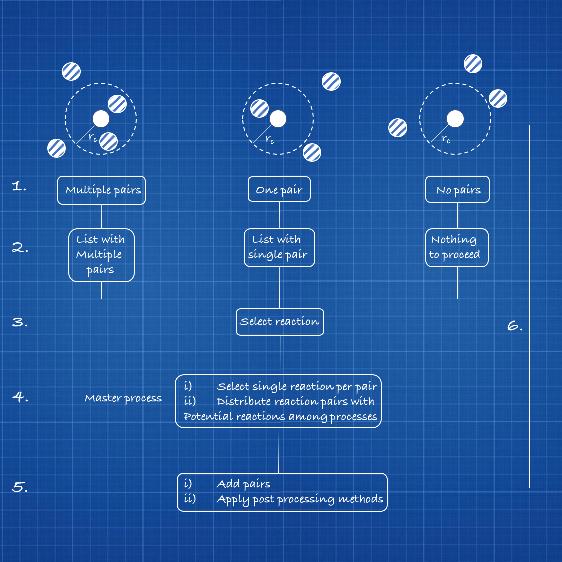
As displayed in figure 1, the first step of the simulation is setting up the particles in a reaction space. For this, a Lennard-Jones potential is used to give all particles the ability to recognize other particles in a specific cut-off radius (rc)[1.]
Then, the algorithm generates a list of all the potential binding partners [2.].
The next step is to select all the possible bonds [3].
After this, one bonding interaction is randomly chosen and the bonding potential is determined [4]. The bond between the particles is finally fulfilled and post process methods are applied. These include a reset of the bond list, a redefining of binding affinity potentials of the new build particle groups, and a characterization of ghost particles, that are already bound to as many particles, as they possibly can.
The ghost particles are then not able to react anymore [5.].
To simulate further polymer chain growth these five steps are looped as many times as there are still particles, that are capable to react [6.].

Figure 1: Display of a theoretical six-step procedure of a molecular dynamic simulation for particle reactions.

However, since there was not enough time to realize this part of the project, we were not able to create the full simulation. But if the MD simulation would have been successful, it would have made a major impact on the optimization of our experimental polymer synthesis. With its results it would have been possible to predict the average chain length and monomer ratio. This would then make it possible to synthesize a predictable polymer.

Team

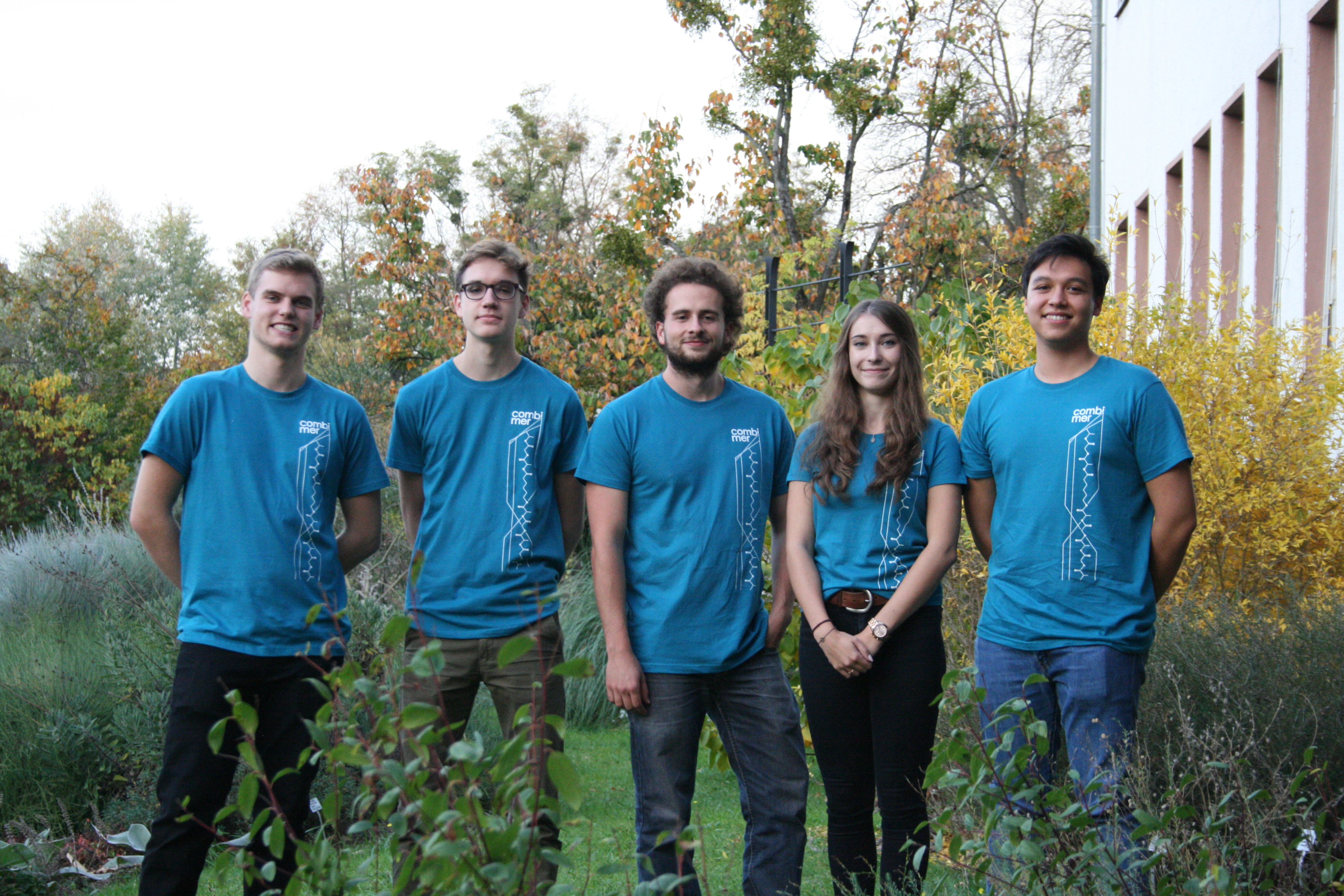
Group picture of the "Modeling" team
From left to right: Luca Brenker, Peter Gockel, Yannick Kristiansen, Jennifer Zimmermann and Jonathan Funk