Difference between revisions of "Team:Valencia UPV/Modeling"
| Line 212: | Line 212: | ||
<div class="col-md-3" style="text-align: center;margin-right: 2em;"> | <div class="col-md-3" style="text-align: center;margin-right: 2em;"> | ||
<a class="inner-link" href="#charact"><img class="fotosModeling" src="https://static.igem.org/mediawiki/2018/c/ca/T--Valencia_UPV--instagramUPV2018.png"></a> | <a class="inner-link" href="#charact"><img class="fotosModeling" src="https://static.igem.org/mediawiki/2018/c/ca/T--Valencia_UPV--instagramUPV2018.png"></a> | ||
| − | <p style="text-align: center !important; font-weight: bold;"> | + | <p style="text-align: center !important; font-weight: bold;">Characterization procedures</p> |
</div> | </div> | ||
<div class="col-md-3" style="text-align: center;margin-right: 2em;"> | <div class="col-md-3" style="text-align: center;margin-right: 2em;"> | ||
| Line 507: | Line 507: | ||
<h6><b>Experiments changing RBS</b></h6> | <h6><b>Experiments changing RBS</b></h6> | ||
<p> | <p> | ||
| − | We have designed <b>two experiments</b> following the same <a href="#exp_protocol" class="inner-link">experimental protocol</a>. In them we have assembled different Printeria TU with the same promoters, CDS and transcriptional terminator, but with <b>different RBS</b>. After obtaining the results, and following the <a href="#optimization" class="inner-link">optimization protocol</a>, we have obtained the parameters of the model and have validated our model. | + | We have designed <b>two experiments</b> following the same <a href="#exp_protocol" class="inner-link">experimental protocol</a>. In them we have assembled different Printeria TU with the same promoters, CDS (<a href="http://parts.igem.org/Part:BBa_K2656013" target="_blank">sfGFP reporter protein</a></b>) and transcriptional terminator, but with <b>different RBS</b>. After obtaining the results, and following the <a href="#optimization" class="inner-link">optimization protocol</a>, we have obtained the parameters of the model and have validated our model. |
</p> | </p> | ||
<p><b>Printeria RBS</b>:</p> | <p><b>Printeria RBS</b>:</p> | ||
| Line 615: | Line 615: | ||
</tr> | </tr> | ||
</table> | </table> | ||
| − | <img src=""> | + | <img src="https://static.igem.org/mediawiki/2018/b/b1/T--Valencia_UPV--optimization_exp1_RBS_graphUPV2018.png"> |
<table style="width:100%"> | <table style="width:100%"> | ||
<tr> | <tr> | ||
<th><p>Optimized parameters</p></th> | <th><p>Optimized parameters</p></th> | ||
| − | <th><p> | + | <th><p>Values</p></th> |
</tr> | </tr> | ||
<tr> | <tr> | ||
| Line 800: | Line 800: | ||
<a class="anchorOffset" id="charact"></a> | <a class="anchorOffset" id="charact"></a> | ||
| − | <h3> | + | <h3>Characterization procedures</h3> |
<p> | <p> | ||
| − | This year, Valencia UPV iGEM team has designed an extensive <a href="https://2018.igem.org/Team:Valencia_UPV/Part_Collection" target="_blank">Part Collection </a> in purpose of allowing the user to design multiple genetic constructions and experiments. One of our main objectives has been to <b>show the user clear and structured information</b> about the pieces that make up the Printeria kit. For this reason, we have considered the characterization of the parts as a priority when developing the project. In this way, we have elaborated some <b>procedures</b> which have allowed us to systematically obtain and structure information from the parts. | + | This year, Valencia UPV iGEM team has designed an extensive <a href="https://2018.igem.org/Team:Valencia_UPV/Part_Collection" target="_blank">Part Collection</a> in purpose of allowing the user to design multiple genetic constructions and experiments. One of our main objectives has been to <b>show the user clear and structured information</b> about the pieces that make up the Printeria kit. For this reason, we have considered the characterization of the parts as a priority when developing the project. In this way, we have elaborated some <b>procedures</b> which have allowed us to systematically obtain and structure information from the parts. |
<ul> | <ul> | ||
<li><p> | <li><p> | ||
Revision as of 17:18, 5 October 2018

Modeling
Do you think it is possible to mathematically describe a cell? Would you like to know the possibilities that Printeria modeling offers you?
One of the fundamental bases of the Printeria project has undoubtedly been mathematical modeling. Thanks to the development and application of new mathematical models, it is possible to quantify the expression of proteins in cells, and therefore characterize through different experiments the parts designed by Printeria. From the Printeria modeling team, we intend to reach different goals:
Design simple mathematical models based on differential equations that describe the biochemical processes of a cell. With them, we can simulate the different genetic circuits that Printeria allows us to build.
Develop a Simulation Tool that allows the user to visualize a prediction of the results of their experiment before running it in Printeria.
Optimize model parameters to match simulation results to experimental data obtained from Printeria constructions.
Characterize the parts of our Part Collection from the optimization results and provide the user with all the information about the Printeria kit.
Although in the development of the project we have dealt with all these aspects, all of them have a single purpose: to understand and describe in a mathematical way the biological processes that take place inside the cell.

Models & Experiments
Characterization procedures
Simulation Tool
Models & Experiments
The development of new and simple mathematical models has been one of the essential bases of the Printeria project. The models offer us a multitude of applications: to describe the basic biochemical reactions of the cell, to characterize the parts of our Printeria kit by means of different experiments or to elaborate new tools that facilitate to our user the learning of Synthetic Biology.
In Printeria Modeling team, we have grouped the models designed in two fields: constitutive expression models and inducible expression models. We have also established an experimental protocol and a multi-objective optimization protocol in order to contrast theoretical and experimental results. With them, we can describe practically all the cells modified with Printeria.
Want to find out more about how we did it?
Modeling process
At the beginning of the design of any mathematical model, we have started from a cell scheme in which all the cellular biochemical reactions we wish to model are represented. From the reactions, a set of equations is deduced. Each of these equations describes the temporal variation of the biochemical species in the cell (DNA, RNA, proteins...), and depends on a set of parameters with a physical meaning.
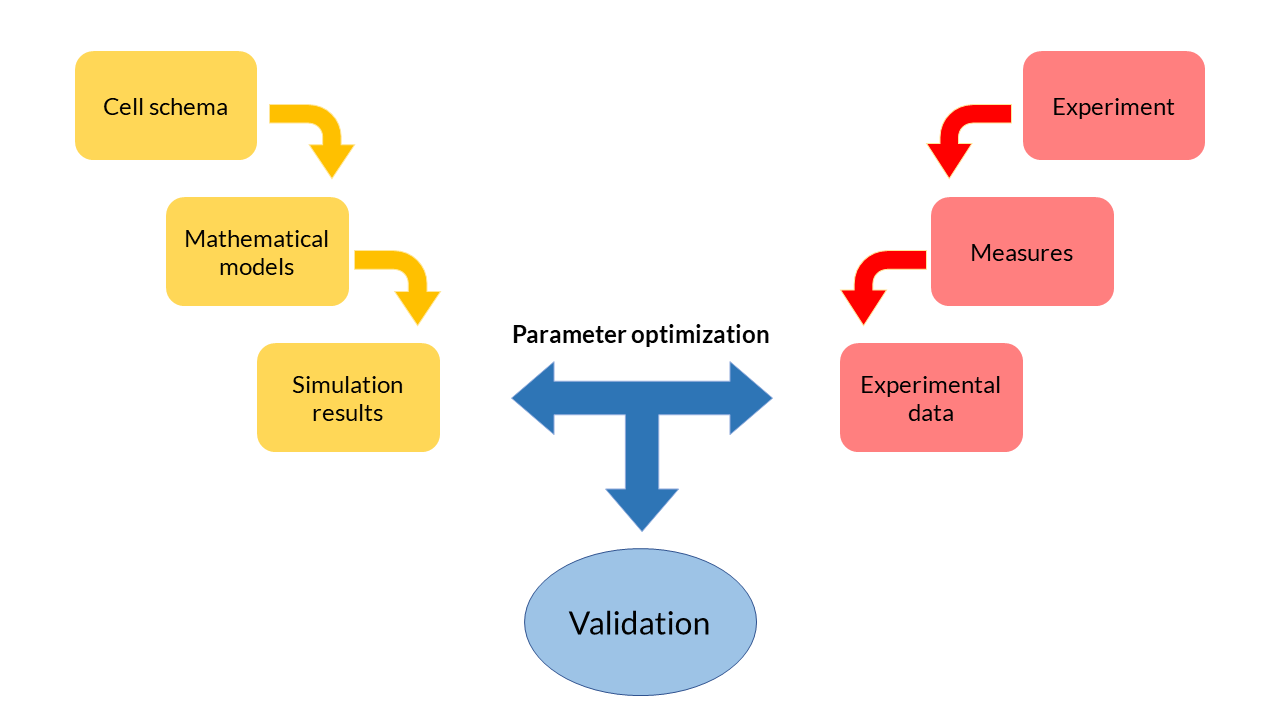
Because they are differential and generally non-linear equations, mathematical models are simulated using software tools such as MATLAB. The results obtained from the simulation reflect the evolution of the concentration of biochemical species over time. These theoretical results can be contrasted with the experimental data obtained in the laboratory and and thereby adjust the parameters so that the model adapts to the data in an optimal way. This process, called multiobjective parameter optimization, is the process that allows us to validate our models and see if they respond to what happens inside the cells.
In the development of the set of mathematical models that describe the genetic circuits printed by Printeria, we have prioritized simplicity over complexity of the model. A more complex model may be more precise, but it requires a large number of parameters whose value is often unknown. Therefore, our models are composed of few equations and parameters, and they are all deterministic models, that is, their parameters take a concrete, non-probabilistic value.
Experimental protocol
The Printeria Modeling and Lab team and have jointly designed an experimentation protocol for the laboratory experiments. Thanks to it, and from the colonies of the different UT the experimental data can be obtained, processed and ready to be optimized.
Materials:
-
Printeria transcriptional units (see our Printeria Part Collection)
-
Measuring equipment: Biotek Cytation3
-
96 well plate
-
MATLAB 2018a software
Protocol:
The TU colonies assembled by our Lab team are diluted in the medium (generally we have used LB or M9 medium with Kanamycin) so that they all have the same OD.
The experiment is designed on the measuring equipment. In our case, we use the Biotek Cytation3 equipment. We establish the equipment parameters.
Parameters
Description
Time
06:00:00 (HH:MM:SS) usually. Measurement interval: 05:00 (MM:SS)
Number of samples
We normally set 8 samples of reporter protein for each TU colony
Number of medium samples
We normally set 8 samples of medium. We normally use LB or M9 medium with Kanamycin
Temperature
37 ºC
Shake
Double Orbital. Continuously. We shake the plate before each measure
Absorbance. Optical Density (OD) measure
Wavelenght at 600 nm emission
Excitacion wavelength
We normally set 485 nm
Emission wavelength
We normally set 528 nm
Gain (G)
Normally the gain value is G = 60, although for proteins with lower fluorescence, it is recommended that G takes higher values.
Samples are introduced into the 96 well plate and the experiment begins.
After the experiment, fluorescence and absorbance data obtained are exported to an Excel file.
We run the MATLAB convert_data.m script. This script uses several additional MATLAB files with which:
We extract the fluorescence and absorbance matrices from the Excel file (see readExperiment3.m MATLAB function).
We apply the corrections to the data (see plotExperiment_yb.m MATLAB function).
We save the data of FOD, OD, molecules and time in a .mat format file.
Multi-objective parameter optimization
To what extent is our model valid? What values should the parameters take? To what extent do the theoretical results resemble the experimental ones? Is our model able to explain the behaviour of cells in reality?
One of the most important phases in the field of Printeria Modeling has been the validation of theoretical models with experimental data. In the Printeria team we wanted to confirm that the models designed are consistent with our experiments. However, we know that the parameters will not take a fixed value, but vary depending on the genetic construction with which we experiment. With this idea in mind, the need to apply an optimization process arises.
The process of multiobjective parameter optimization consists in finding those parameters of the model that best fit a particular objective, i.e., a particular set of experimental data. From a dataset, and applying a mathematical algorithm, we can find the optimal solutions, also known as Pareto-optimal or Pareto front solutions. These solutions are such that there are no more solutions that do not improve one objective without worsening the rest.
From the Printeria Modeling team we have established a protocol that allows us to obtain the optimal solutions of the model parameters for any experiment:
We define the objectives to be optimized. These will be the values of Fluorescence F/Unit of Absorbance OD or FOD, and the cellular growth (OD) of a Transcriptional Unit (TU). Therefore, if we have different n TU in an experiment, we will optimize 2n objectives.
We choose the parameters to optimize and establish the range of values they can take.
We select the identification and validation data. The identification data are those used in the optimization process. The validation data are used to compare the experiment with the simulated theoretical model and the optimized parameters.
We define the cost function, which specifies the error function to be minimized, simulates the model with different parameter values, and calculates the error between the simulation data and the experimental identification data.
The mathematical optimization algorithm is executed. In our case we use the Multi-objective Differential Evolution Algorithm with Spherical Pruning. This algorithm uses the cost function to test different parameter values and thus search for optimal parameter values.
The Pareto set and Pareto Front diagrams and the different solutions of our optimized parameters for the different objectives are obtained.
Decision Making is carried out by the designer. The optimal parameters are chosen for our 2n objectives.
The model is simulated with the optimized parameters and compared with the validation data.
Following this protocol, and particularizing it for each experiment, we have been able to determine the validity of our models and obtain the best parameters for our experiments.
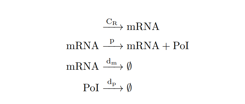
Constituve expression models
Constitutive expression models are those in which the expression of the cell's messenger RNA (mRNA) is not regulated. The gene does not depend on any inducing biochemical species, so it will produce RNA molecules continuously, and therefore the translation of the protein will also be constant.
Model design
A simple scheme that summarizes the cellular transcription and translation processes in a constitutive expression model is shown in the following Figure. We only consider as biochemical species involved in reactions to mRNA and our protein of interest (PoI).
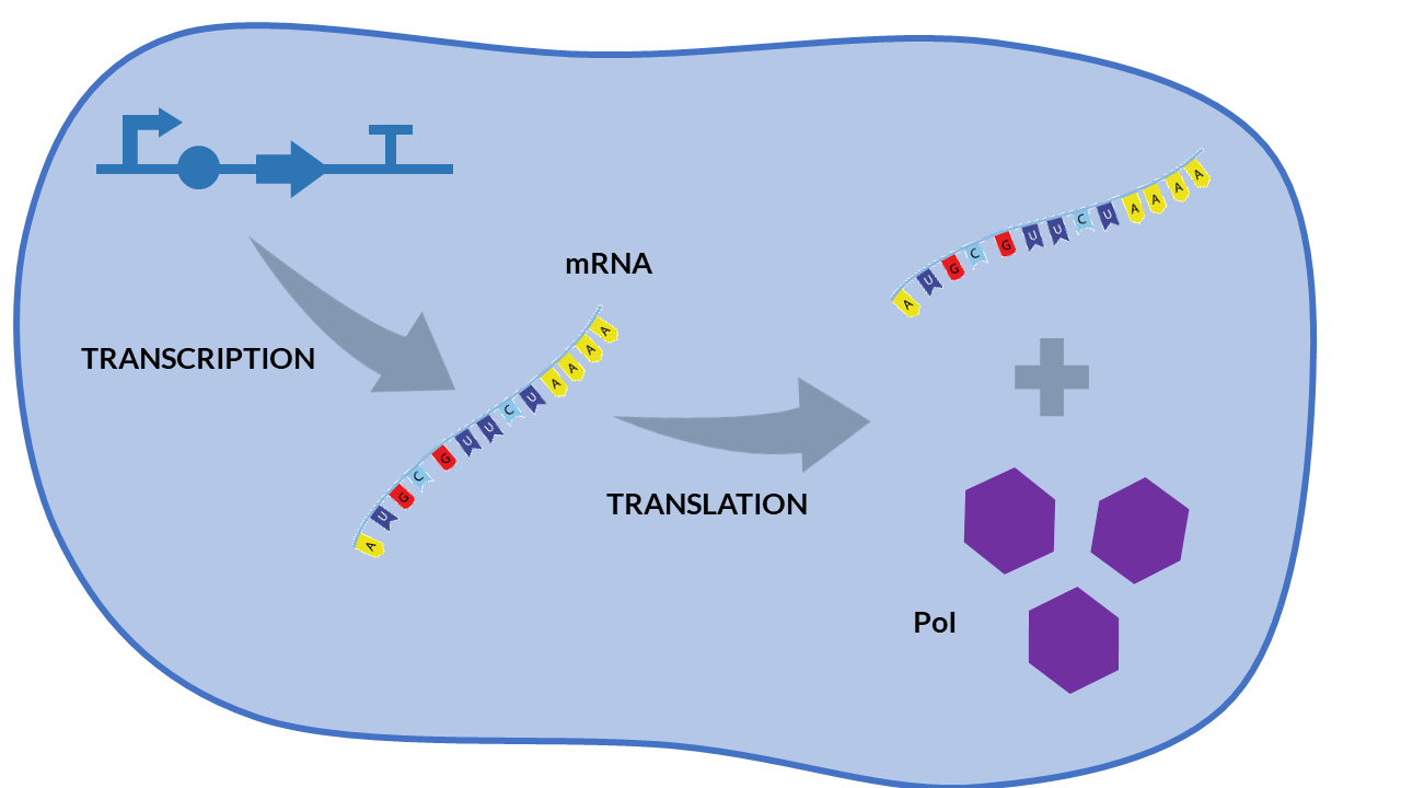
From the cell schema, we can deduce the following biochemical reactions.
Parameter |
Description |
Units |
Value |
|---|---|---|---|
CR |
Constitutive transcription rate |
molecules.min-1 |
|
p |
Translation rate |
min-1 |
|
dm |
mRNA degradation rate |
min-1 |
|
dp |
PoI degradation rate |
min-1 |
|
μ |
Dilution rate |
min-1 |
|
Kmax |
Maximum growth capacity |
cells |
With the reactions and approximations already established, we apply the Law of Mass Action kynetics (LMA) to deduce the differential equations. The LMA establishes that the variation of the species resulting from a reaction is proportional to the product of the reactants. In our case, to the set of differential equations deduced from the reactions we add a cell growth equation. Biochemical species and our model of equations obtained are shown below.
Variable |
Biochemical species |
Units |
|---|---|---|
n1 |
mRNA |
Molecules |
n2 |
PoI |
Molecules |
n3 |
Number of cells |
Cells |
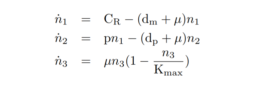
By obtaining the equations, and seeking the simplicity of the model, a series of quasi-static approximations have been made. We have established that mRNA is generated with a constant CR constitutive transcription rate. Another consideration has been to assume that the copy number of plasmids in cell is constant. We have also proposed that other species such as ribosomes, which also participate in transcription, are constant over time.
After developing the model and raising the reactions and equations, two files have been programmed in MATLAB: the mc_simple.m function, which describes the system of differential equations, and the script model_const_simple.m in which the parameters are defined and the model is solved by the ode45 MATLAB function. The result of the simulation of the model is shown in the following Figure.
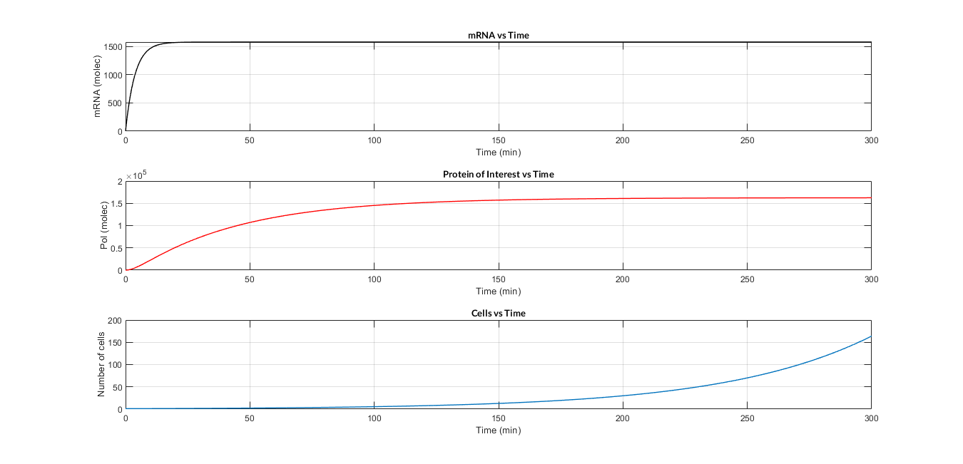
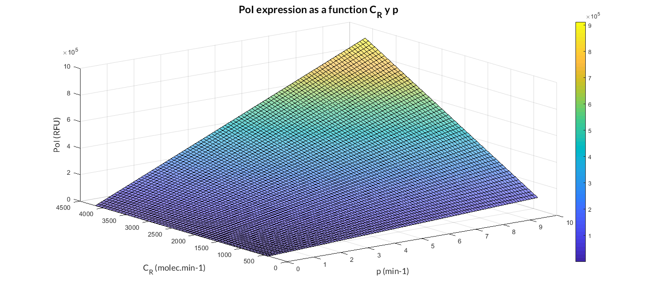
In the simulation of mRNA and PoI we distinguish two phases in the temporal evolution of the species: the transient phase and the stationary phase. If we perform different simulations varying some parameters of the model, we can observe how the equilibrium value of the stationary phase varies. MATLAB script mc_sim_analysis.m repeatedly simulates the model by varying the CR and p parameters, and graphs the results. The following Figure shows how an increase in both ratios implies a greater expression of the protein.
At this point anyone could ask us: Which are the advantages of a constitutive expression model like this? Why is a model like this really useful to us? Faced with these questions, the Printeria Modeling team has looked for the answers in the great characteristics that the model offers us.
A simple, easy-to-understand model that clearly explains the processes of cellular transcription and translation.
It is valid for any Printeria construction that has a constitutive expression promoter. The variation between different constructions occurs in the parameters values, not in the model equations!
It has few parameters, with a clear physical meaning, and easily optimizable.
As a compact model, simulations and optimizations are performed at high speed.
Experiments & optimization
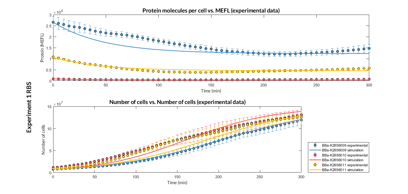
The simple model of constitutive expression is a model that characterizes a large number of Printeria Transcriptional Units (TU), specifically, all those constructions whose promoter is constitutive. We know that all these TU follow the same model, but each one has different parameters, and therefore different experimental values of fluorescence and absorbance. Faced with this situation, the Printeria Lab and Modeling teams have designed some experiments changing RBS and promoters, in which we have applied the multi-objective parameter optimization, and thus check whether the designed constitutive expression model responds to experimental reality.
Experiments changing RBS
We have designed two experiments following the same experimental protocol. In them we have assembled different Printeria TU with the same promoters, CDS (sfGFP reporter protein) and transcriptional terminator, but with different RBS. After obtaining the results, and following the optimization protocol, we have obtained the parameters of the model and have validated our model.
Printeria RBS:
Strong expression: BBa_K2656009.
Medium expression: BBa_K2656011.
Low expression: BBa_K2656010.
Very low expression: BBa_K2656008, BBa_K2656012.
Experiment parameters |
Description |
|---|---|
Time |
06:00:00 (HH:MM:SS). Measurement interval: 05:00 (MM:SS) |
Number of samples |
8 samples for each TU colony |
Number of medium samples |
8 samples of M9 medium |
Temperature |
37 ºC |
Shake |
Double Orbital. Continuously |
Absorbance. Optical Density (OD) measure |
Wavelenght at 600 nm emission |
Excitacion wavelength |
Wavelenght at 485 nm |
Emission wavelength |
Wavelenght at 528 nm |
Gain (G) |
60 |
Optimization specifications |
Description |
|---|---|
Parameters |
Constitutive transcription rate (CR): fixed Translation rate (p): to optimize PoI degradation rate (dp): to optimize mRNA degradation rate (dp): fixed Dilution rate (μ): to optimize Maximum growth capacity (Kmax): experimental value |
Objetives to optimize |
For each TU, we set 2 objetives: FOD (Fluorescence) and OD (Absorbance). In each experiment we have measured 3 TU, so we must set 6 objectives par experiment |
Parameter ranges |
Translation rate (p): [0.001 - 6] min-1 PoI degradation rate (dp): [0.0058 - 0.0087] min-1 Dilution rate (μ): [0.0058 - 0.035] min-1 |
MATLAB files |
spMODEparam.m: it defines the parameters to be optimized, their value ranges, number of objectives, the cost function, the identification and validation experimental data and other spMODE algorithm parameters. When the script is executed, a spMODEDat structure variable is defined. This structure contains all the standardized optimization information that the spMODE algorithm will need for its execution.
spMODE.m: it contains the Multi-objective Differential Evolution Algorithm with Spherical Pruning, which optimizes parameters for our experimental results (to execute spMODE.m file we need also SphPruning.m file). CostFunction_XFP_RMS_2n.m: it simulates the model with different vector parameters, and calculates the Root Mean Square Error with the identification dataset. Then, it returns the error for each objective and parameter vector. levelDiagram.m: plots Pareto front and Pareto set that gives us back the algorithm. execute.m: this script launches the optimization by executing spMODEparam.m, spMODEm algorithm and levelDiagram.m. Then, allows the user to enter the best parameters, and plots validation experimental data and simulation results in the same graph. |
Optimized parameters |
Values |
|---|---|
Translation rate p |
Experiment 1:
Experiment 2:
|
PoI degradation rate dp |
Experiment 1: dp = 0.0058 min-1 Experiment 2: dp = - min-1 |
Dilution rate μ |
Experiment 1:
Experiment 2:
|
Experiments changing promoters
We have designed two experiments following the same experimental protocol. In them we have assembled different Printeria TU with the same RBS, CDS and transcriptional terminator, and with different promoters. After obtaining the results, and following the optimization protocol, we have obtained the parameters of the model and have validated our model.
Printeria TU:
Strong promoters:pITU 6 20 21 (ADD REFERENCES)
Medium promoters:
Low promoters:
Experiment parameters |
Description |
|---|---|
Time |
06:00:00 (HH:MM:SS). Measurement interval: 05:00 (MM:SS) |
Number of samples |
8 samples for each TU colony |
Number of medium samples |
8 samples of M9 medium |
Temperature |
37 ºC |
Shake |
Double Orbital. Continuously |
Absorbance. Optical Density (OD) measure |
Wavelenght at 600 nm emission |
Excitacion wavelength |
Wavelenght at 485 nm |
Emission wavelength |
Wavelenght at 528 nm |
Gain (G) |
60 |
Optimization specifications |
Description |
|---|---|
Parameters |
Constitutive transcription rate (CR): to optimize Translation rate (p): fixed PoI degradation rate (dp): to optimize mRNA degradation rate (dp): fixed Dilution rate (μ): to optimize Maximum growth capacity (Kmax): experimental value |
Objetives to optimize |
For each TU, we set 2 objetives: FOD (Fluorescence) and OD (Absorbance). In each experiment we have measured 3 TU, so we must set 6 objectives par experiment |
Parameter ranges |
Translation rate (p): [0.001 - 6] min-1 PoI degradation rate (dp): [0.0058 - 0.0087] min-1 Dilution rate (μ): [0.0058 - 0.035] min-1 |
MATLAB files |
spMODEparam.m: it defines the parameters to be optimized, their value ranges, number of objectives, the cost function, the identification and validation experimental data and other spMODE algorithm parameters. When the script is executed, a spMODEDat structure variable is defined. This structure contains all the standardized optimization information that the spMODE algorithm will need for its execution.
spMODE.m: it contains the Multi-objective Differential Evolution Algorithm with Spherical Pruning , wich optimizes parameters for our experimental results (to execute spMODE.m file we need also SphPruning.m file).CostFunction_XFP_RMS_2n.m: it simulates the model with different vector parameters, and calculates the Root Mean Square Error with the identification dataset. Then, it returns the error for each objective and parameter vector. levelDiagram.m: plots Pareto front and Pareto set that gives us back the algorithm. execute_2n.m: this script launches the optimization by executing spMODEparam.m, spMODEm algorithm and levelDiagram.m. Then, allows the user to enter the best parameters, and plots validation experimental data and simulation results in the same graph. |
Inducible expression models
Characterization procedures
This year, Valencia UPV iGEM team has designed an extensive Part Collection in purpose of allowing the user to design multiple genetic constructions and experiments. One of our main objectives has been to show the user clear and structured information about the pieces that make up the Printeria kit. For this reason, we have considered the characterization of the parts as a priority when developing the project. In this way, we have elaborated some procedures which have allowed us to systematically obtain and structure information from the parts.
Procedure for obtaining protein spectra
Obtaining excitation and emission spectra is a fundamental aspect in the process of characterization of a fluorescent protein. Each protein has a characteristic spectrum, which indicates the energy in which the molecule is excited or emits at a certain wavelength.
The characterization of the reporter proteins by excitation and emission spectra are of great importance in experimentation. When contrasting experimental information with the theoretical results of mathematical models, we experiment with numerous reporter proteins, such as fluorescence proteins or chromoproteins. However, the fluorescence data obtained must be corrected applying diferent operations in order to obtain representative fluorescence data:
The subtraction of the medium fluorescence:

The quotient of the fluorescence with the gain:

The quotient of the fluorescence with excitation and emission efficiency:


Until now, the corrections applied to the experiments performed with these reporter proteins were the subtraction of the fluorescence of the medium, and the division by the gain factor of the measuring equipment. However, with the protein spectra we can also normalize the fluorescence data to values that would have been obtained with maximum excitation and emission.
Owing to this reason, a protocol has been established in the lab by Lab and Modeling team to obtain the spectrum of any reporter protein.
Materials:
-
Measuring equipment: Biotek Cytation3
-
96 well plate
-
MATLAB 2018a software
Procedure:
We look for the theoretical spectra of the protein to be measured or similar molecules in order to determine the wavelength at which the protein is excited or emitted at maximum energy, i.e. where the theoretical spectral peaks occurs.
We define the protocol of our equipment to get the absorbance and fluorescence dataset. In our protocol, the most important parameters to be established are summarized in the following Table.
Parameters
Description
Number of samples
From 3 to 6 samples of reporter protein and 3 samples of medium (LB or M9 medium)
Temperature
37 ºC
Shake
Double Orbital. 01:00 (MM:SS)
Absorbance. Optical Density (OD)
Wavelenght at 600 nm emission
Excitacion and emission scans
The scans occur between two wavelength limit values. The established range will depend on the theoretical spectrum of the protein.
Excitacion and emission wavelengths
These values will depend on the range, and therefore on the spectrum. Values far from the theoretical peak lead to more attenuated fluorescence curves, and values very close to the peak can lead to overlap and error in reading the data. Therefore, a compromise must be reached between curve resolution and reading overlap.
Gain (G)
Normally the gain value is G = 60, although for proteins with lower fluorescence, it is recommended that G takes higher values.
The experiment is introduced, and the experimental absorbance data and the fluorescence curves of the samples are obtained with the medium fluorescence correction applied.
The dataset is exported to an Excel file.
The MATLAB script spectrum.m for fluorescent proteins is executed:
-
Dataset is extracted from the Excel file. We discard readings that have suffered overlap, or that take negative values.
-
The fluorescence curves of all samples are averaged, and the result is normalised (from 0 to 100%).
-
Graphs of the normalized absorption and emission spectra are plotted. The X-axis represents the wavelength (nm), and the Y-axis represents the normalized fluorescence intensity (%).
-
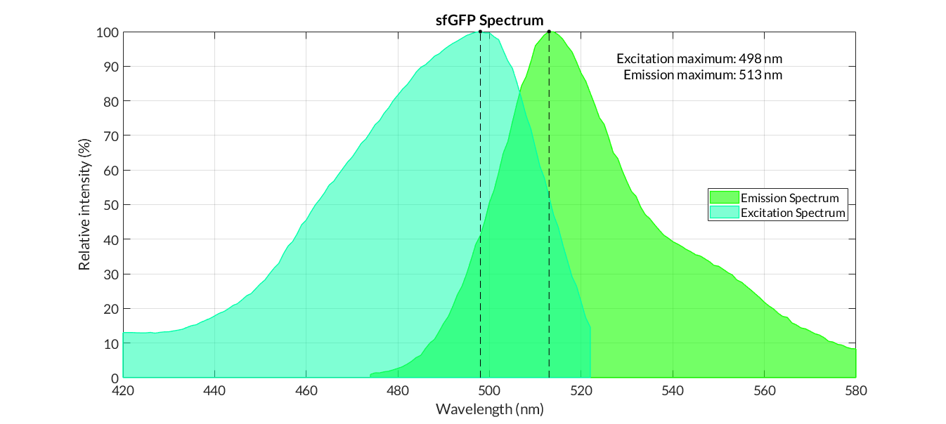
In practical terms, the protocol has been applied to all of our reporter proteins: GFP, sfGFP, YFP and mRFP. All results can be found in our parts collection as well as in the iGEM catalog.
In the particular case of a reporter chromoprotein, such as amilCP, we do not measure fluorescence, but absorbance. In this case, in rder to obtain the corrected absorbance curve, we must subtract from the cell absorbance data with the reporter protein the absorbance of a medium with cells without chromoprotein. Once the data have been corrected, we normalize them between values of 0 and 100 and with this we elaborate the graph. The protocol used can be found in the MATLAB script amilCP_spectrum.m.
Finally, we have also obtained the spectra of the fluorescein molecule. These spectra have been used to correct the fluorescence data used in the Interlab Study to obtain the Relative Fluorescence Units (RFU) to Molecules of Equivalent Fluorochrome (MEFL) conversion factor. In addition, the comparison between GFP and sfGFP proteins RFU has been possible thanks to fluorescein spectra.
Parameters |
Value |
|---|---|
Number of samples |
6 samples. 3 samples of medium (LB or M9 medium) |
Temperature |
37 ºC |
Shake |
Double Orbital. 01:00 (MM:SS) |
Absorbance. Optical Density (OD) |
Wavelenght at 600 nm emission |
Emission range |
[495 - 580] nm |
Fixed excitation wavelength |
480 nm |
Excitation range |
[430 - 520] nm |
Fixed emission wavelength |
545 nm |
Gain (G) |
60 |

Comparison between sfGFP and GFP relative fluorescence intensity
One of the main problems we encounter when processing the results of experiments in Synthetic Biology are the units of measurement of fluorescence data. Unlike absorbance, where there is a simple conversion between Optical Density (OD) and cell number, there is no direct relationship between the Relative Units of Fluorescence (RFU) and the number of protein molecules in the cell. Moreover, RFUs vary among reporter fluoroproteins: for example, an RFU of the GFP protein does not have to be equivalent to an RFU of the mRFP protein, sfGFP, etc.
Thanks to initiatives such as the Interlab Study, we have been able to go a step further and obtain a MEFL/cellGFP factor of equivalence between the RFU of the GFP protein and the Molecules of Equivalent Fluorochrome (MEFL). This relationship is an important breakthrough, as it can give us a more accurate estimation of the amount of GFP molecules in the cell.
However, another reporter protein widely used in the experiments is the sfGFP. This protein has a much faster folding than GFP, which translates into a higher fluorescence intensity per molecule. In order to obtain the MEFL/cellsfGFP factor from sfGFP, the Printeria Modeling and Lab teams have designed a comparative experiment between both proteins. The experiment consists of designing two identical transcriptional units (TU), changing only the CDS sequence so that each TU will produce GFP and sfGFP, respectively. It should be added that this experiment is based on two fundamental assumptions:
The number of GFP molecules produced in the cells is equivalent to the number of MEFL.
Given two TU with identical promoters, RBS and terminators, but with different CDS, under the same experimental conditions, the number of molecules produced by each TU is the same.
Taking these axioms into account, the materials and procedure followed to calculate the MEFL/cellsfGFP factor were as follows.
Materials:
-
Measuring equipment: Biotek Cytation3
-
96 well plate
-
MATLAB 2018a software
Procedure:
From the fluorescein spectrum, and the fluorescence data obtained from the Interlab Study experiment, we apply medium, gain and efficiency corrections .
The data are introduced in the Excel file of the Interlab Study. From the Fluorescein standard curve sheet we can obtain the MEFL/RFU factor, and then calculate the MEFL/cell factor.

Parameters
Value
Cuture volume (96 well plate)
200 μL
Cells per μL per OD unit
200 cells/OD μ L
MEFL/RFU factor
4,38.1010 MEFL/RFU
MEFL/cellGFP factor
273.7 MEFL OD/RFU cell
We establish the protocol of the experiment and the parameters of our equipment. The experiment consists in the measurement of the absorbance and fluorescence of two TU with identical promoter, RBS and transcriptional terminator, but whose CDS codifies for GFP and sfGFP proteins. The most relevant information of the experiment is detailed in the following Table:
Parameters
Description
Time
06:00:00 (HH:MM:SS). Measurement interval: 05:00 (MM:SS)
Number of samples
8 samples for each TU. Total samples: 16
Temperature
37 ºC
Shake
Double Orbital Continuous
Absorbance. Optical Density (OD)
Wavelenght at 600 nm emission
Excitacion wavelength
485 nm
Emission wavelength
528 nm
Gain
60
The experiment is introduced into the equipment and the absorbance and fluorescence curves are obtained, as well as the curve of Fluorescence F/Absorbance OD or FOD ratio with the applied medium fluorescence correction.
The absorbance and fluorescence data are exported to an Excel file.
Running the MATLAB GFP_sfGFP_comparison.m script:
-
We extract the FOD data from the GFP and sfGFP from the Excel file.
-
We apply the gain and efficiency corrections of the spectrum to the FOD.
-
We plot the FOD curves and look for a stationary equilibrium time interval in the expression of the GFP and sfGFP proteins. In our experiment, we have decided to chose the interval [145,290] min
-
We obtain the average value of both regions.
-
We calculate the number of GFP MEFLs by multiplying the FOD data by the MEFL/cellGFP factor.
-
If we assume that the number of molecules expressed by both TU is the same, the number of MEFL for the calculated GFP is the same as the number of MEFL for the sfGFP.
-
We calculate the MEFL/cellsfGFP factor by dividing the MEFL number by the average FOD value of the sfGFP in the stationary region. In our case, MEFL/cellsfGFP = 121.4 MEFL·OD/RFU·cell.
-

Reporter protein |
MEFL/cell factor (MEFL·OD/RFU·cell) |
|---|---|
GFP |
273.7 |
sfGFP |
121.4 |
With MEFL/cell factors, FOD data obtained in any experiment in which GFP or sfGFP was used as reporter proteins can be transformed into equivalent fluorescein molecules by applying the following ratio: Molecules = (MEFL/cell factor) · FOD.
The new data give us a more accurate estimation of the number of molecules in the cell. Consequently, by relating the experimental results with the theoretical mathematical models in the optimization process, the parameters of the model acquire values more consistent with their physical significance, working in equivalent molecules and not in arbitrary units.
Simulation Tool