Team:Valencia UPV/Model


Modeling
Do you think it is possible to mathematically describe a cell? Would you like to know the possibilities that modeling offers you?
One of the fundamental bases of the Printeria project has undoubtedly been mathematical modeling. Thanks to the development and application of new mathematical models, it is possible to quantify the expression of proteins in cells, and therefore characterize through different experiments the parts designed by Printeria. From the Printeria Modeling team, we intend to reach different goals:
Design simple mathematical models based on differential equations that describe the biochemical processes of a cell. With them, we can simulate the different genetic circuits that Printeria allows us to build.
Develop a Simulation Tool that allows the user to visualize a prediction of the results of their experiment before running it in Printeria.
Optimize model parameters to match simulation results to experimental data obtained from Printeria constructions.
Characterize the parts of our Part Collection from the optimization results and provide the user with all the information about the Printeria kit.
Although in the development of the project we have dealt with all these aspects, all of them have a single purpose: demonstrate the importance and many applications of describing in a mathematical way the biological processes that take place inside the cell.
Models & Experiments
The development of new and simple mathematical models has been one of the essential bases of the Printeria project. The models offer us a multitude of applications: to describe the basic biochemical reactions of the cell, to characterize the parts of our Printeria kit by means of different experiments or to elaborate new tools that facilitate to our user the learning of Synthetic Biology.
In Printeria Modeling team, we have grouped the models designed in two fields: constitutive expression models and inducible expression models. We have also established an experimental protocol and a multi-objective optimization protocol in order to contrast theoretical and experimental results. With them, we can describe practically all the cells modified with Printeria.
Want to find out more about how we did it?
Modeling process
At the beginning of the design of any mathematical model, we have started from a cell scheme in which all the cellular biochemical reactions we wish to model are represented. From the reactions, a set of equations is deduced. Each of these equations describes the temporal variation of the biochemical species in the cell (DNA, RNA, proteins...), and depends on a set of parameters with a physical meaning.
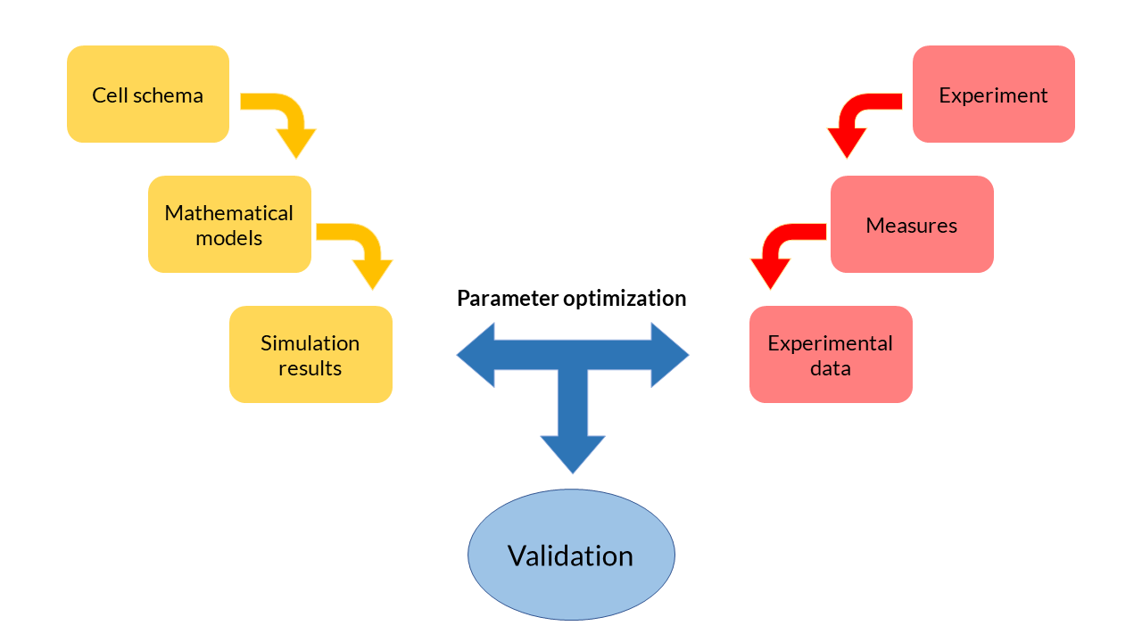
Modeling process schema.
Because they are differential and generally non-linear equations, mathematical models are simulated using software tools such as MATLAB. The results obtained from the simulation reflect the evolution of the concentration of biochemical species over time. These theoretical results can be contrasted with the experimental data obtained in the laboratory and and thereby adjust the parameters so that the model adapts to the data in an optimal way. This process, called multiobjective parameter optimization, is the process that allows us to validate our models and see if they respond to what happens inside the cells.
In the development of the set of mathematical models that describe the genetic circuits printed by Printeria, we have prioritized simplicity over complexity of the model. A more complex model may be more precise, but it requires a large number of parameters whose value is often unknown. Therefore, our models are composed of few equations and parameters, and they are all deterministic models, that is, their parameters take a concrete, non-probabilistic value.
Constitutive expression models
Constitutive expression models are those in which the expression of the cell's messenger RNA (mRNA) is not regulated. The gene does not depend on any inducing biochemical species, so it will produce RNA molecules continuously, and therefore the translation of the protein will also be constant.
Model design
A simple scheme that summarizes the cellular transcription and translation processes in a constitutive expression model is shown in the following Figure. We only consider as biochemical species involved in reactions to mRNA and our protein of interest (PoI).
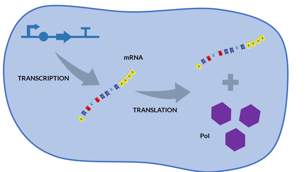
Constitutive expression model. Cell schema.
From the cell schema we can deduce the following biochemical reactions.
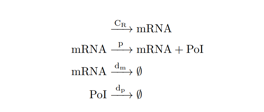
Constitutive expression model. Biochemical reactions.
Parameter |
Description |
Units |
Value |
|---|---|---|---|
CR |
Constitutive transcription rate is the transcription rate KR times the mean plasmid copy number in cell cn. In our case, we are using the pMBI replication origin, so cn ∼ 500, and CR = KR·cn |
molecules.min-1 |
|
p |
Translation rate |
min-1 |
2.38 [2] |
dm |
mRNA degradation rate |
min-1 |
0.247 [7] |
dp |
PoI degradation rate |
min-1 |
0.156 [5] |
μ |
Dilution rate |
min-1 |
0.017 [5] |
Kmax |
Maximum growth capacity |
cells |
1.6·108 [5] |
Constitutive expression model. Model parameters obtained from literature.
With the reactions and approximations already established, we apply the Law of Mass Action kynetics[1] (LMA) to deduce the differential equations. The LMA establishes that the variation of the species resulting from a reaction is proportional to the product of the reactants. In our case, to the set of differential equations deduced from the reactions we add a cell growth equation. Biochemical species and our model of equations obtained are shown below.
Variable |
Biochemical species |
Units |
|---|---|---|
n1 |
mRNA |
Molecules |
n2 |
PoI |
Molecules |
n3 |
Number of cells |
Cells |
Constitutive expression model. Biochemical species.
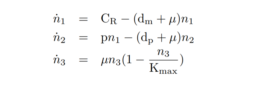
Constitutive expression model. Model equations.
By obtaining the equations, and seeking the simplicity of the model, a series of quasi-steady state approximations [2] have been made. We have established that mRNA is generated with a constant CR constitutive transcription rate. Another consideration has been to assume that the copy number of plasmids cn in cell is a constant. We have also proposed that other species such as ribosomes, which also participate in transcription, are constant over time.
After developing the model and raising the reactions and equations, two files have been programmed in MATLAB: the mc_simple.m function, which describes the system of differential equations, and the script model_const_simple.m in which the parameters are defined and the model is solved by the ode45 MATLAB function. The result of the simulation of the model is shown in the following Figure.
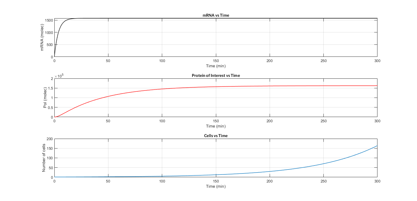
Constitutive expression model. Model predictions using parameter values from literature.
In the simulation of mRNA and PoI we distinguish two phases in the temporal evolution of the species: the transient phase and the stationary phase. If we perform different simulations varying some parameters of the model, we can observe how the equilibrium value of the stationary phase varies. MATLAB script mc_sim_analysis.m repeatedly simulates the model by varying the CR and p parameters, and graphs the results. The following Figure shows how an increase in both ratios implies a greater expression of the protein.
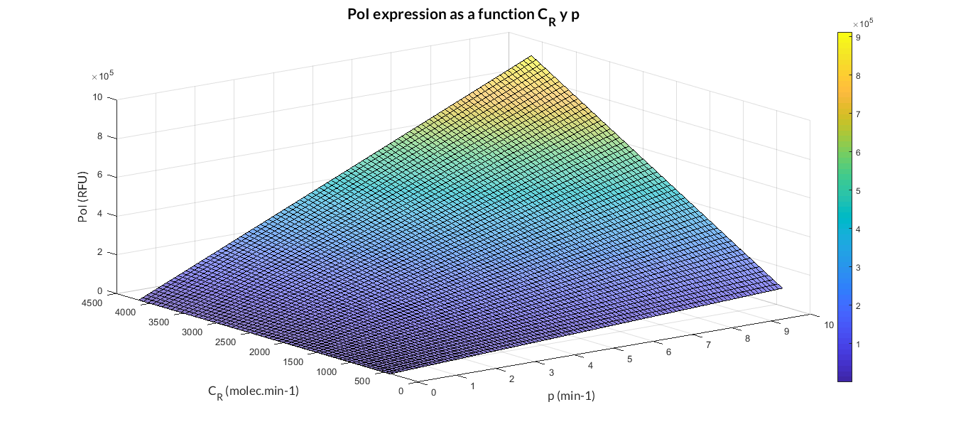
Constitutive expression model analysis. The graph represents de PoI stationary value as function of CR and p ratios.
At this point anyone could ask us: Which are the advantages of a constitutive expression model like this? Why is a model like this really useful to us? Faced with these questions, the Printeria Modeling team has looked for the answers in the great characteristics that the model offers us.
A simple, easy-to-understand model that clearly explains the processes of cellular transcription and translation.
It is valid for any Printeria construction that has a constitutive expression promoter. The variation between different constructions occurs in the parameters values, not in the model equations!
It has few parameters, with a clear physical meaning, and easily optimizable.
As a compact model, simulations and optimizations are performed at high speed.
Experiments & Optimization
The simple model of constitutive expression is a model that characterizes a large number of Printeria Transcriptional Units (TU), specifically, all those constructions whose promoter is constitutive. We know that all these TU follow the same model, but each one has different parameters, and therefore different experimental values of fluorescence and absorbance. Faced with this situation, the Printeria Lab and Modeling teams have designed some experiments, in which we have applied the multi-objective parameter optimization, and thus check whether the designed constitutive expression model responds to experimental reality.
We have designed two experiments following the same experimental protocol. In them we have assembled different Printeria TU with the same promoters, CDS (sfGFP reporter protein) and transcriptional terminator, but with different RBS. After obtaining the results, and following the optimization protocol, we have obtained the parameters of the model and have validated our model.
Printeria RBS:
Strong expression: BBa_K2656009.
Medium expression: BBa_K2656011.
weak expression: BBa_K2656010.
Very weak expression: BBa_K2656008, BBa_K2656012.
Experiment parameters |
Description |
|---|---|
Time |
06:00:00 (HH:MM:SS). Measurement interval: 05:00 (MM:SS) |
Number of samples |
8 samples for each TU colony |
Number of medium samples |
8 samples of M9 medium |
Temperature |
37 ºC |
Shake |
Double Orbital. Continuously |
Absorbance. Optical Density (OD) measure |
Wavelenght at 600 nm emission |
Excitacion wavelength |
Wavelenght at 485 nm |
Emission wavelength |
Wavelenght at 528 nm |
Gain (G) |
60 |
Biotek Cytation 3 experimental parameters.
Optimization specifications |
Description |
|---|---|
Parameters |
Constitutive transcription rate CR: fixed Translation rate p: to optimize PoI degradation rate dp: to optimize mRNA degradation rate dm: fixed Dilution rate μ: to optimize Maximum growth capacity Kmax: experimental value |
Objetives to optimize |
For each TU, we set 2 objetives: FOD (Fluorescence) and OD (Absorbance). In each experiment we have measured 3 TU, so we are optimizing 6 objectives per experiment |
Parameter ranges |
Translation rate p: [0.001 - 6] min-1 PoI degradation rate dp: [0.0058 - 0.0087] min-1 Dilution rate μ: [0.0058 - 0.035] min-1 |
MATLAB files |
spMODEparam.m: it defines the parameters to be optimized, their value ranges, number of objectives, the cost function, the identification and validation experimental data and other spMODE algorithm parameters. When the script is executed, a spMODEDat structure variable is defined. This structure contains all the standardized optimization information that the spMODE algorithm will need for its execution.
spMODE.m: it contains the Multi-objective Differential Evolution Algorithm with Spherical Pruning, which optimizes parameters for our experimental results (to execute spMODE.m file we need also SphPruning.m file). CostFunction_RBS_RMS_2n.m: it simulates the model with different vector parameters, and calculates the Root Mean Square Error with the identification dataset. Then, it returns the error for each objective and parameter vector. levelDiagram.m: plots Pareto front and Pareto set that gives us back the algorithm. execute_RBS_2n.m: this script launches the optimization by executing spMODEparam.m, spMODEm algorithm and levelDiagram.m. Then, allows the user to enter the best parameters, and plots validation experimental data and simulation results in the same graph. |
Optimization specifications for the experiment.
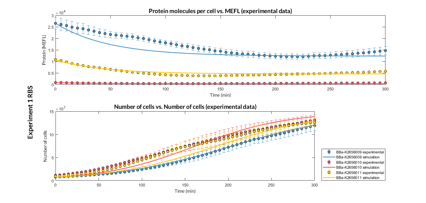
Experiment 1 changing RBS. Experimental and optimized simulated model data of strong, medium and weak protein expression RBS
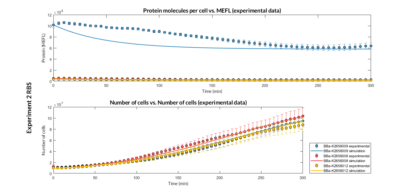
Experiment 2 changing RBS. Experimental and optimized simulated model data of strong and very weak protein expression RBS
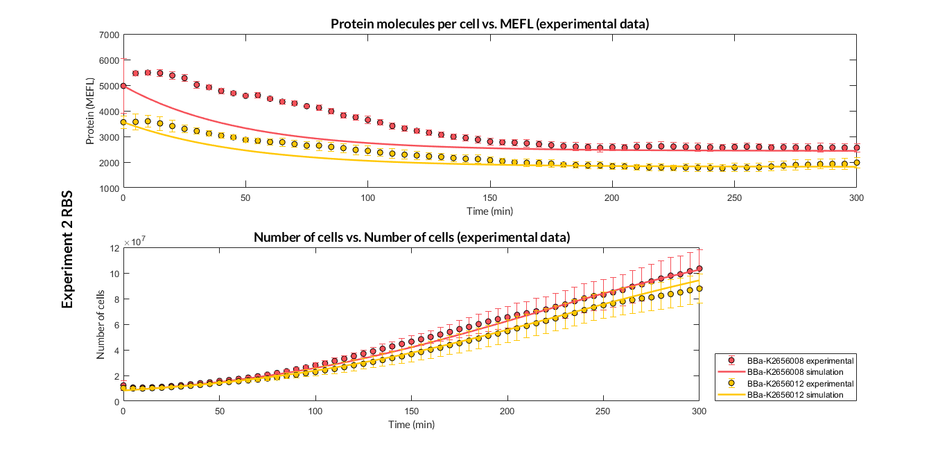
Experiment 2 changing RBS. Experimental and optimized simulated model data of very weak protein expression RBS
The results of the graphs have been obtained after an optimization and decision-making process, in which the optimal parameters have been selected and the constituent model for each objective has been simulated and compared with the experimental data. The optimized parameters are summarized in the following table.
Optimized parameters |
Values |
|---|---|
Translation rate p |
Experiment 1:
Experiment 2:
|
PoI degradation rate dp |
Experiment 1: dp = 0.0058 min-1 Experiment 2: dp = 0.00818 min-1 |
Dilution rate μ |
Experiment 1:
Experiment 2:
|
List of optimized parameters for RBS experiment.
In addition to simulating the optimized models, the Printeria Modeling team has also calculated the relative strength between the different RBS, taking BBa_K2656009 strong RBS as a reference. The relative strength has been defined as the quotient between the values of the protein in equilibrium of the results of the simulation of one RBS and another reference RBS. Likewise, a ratio between p parameters of the different RBS parts and p parameter of the reference RBS has been calculated. The characterization of the RBS parts by their relative strength is shown below.

Original BioBrick RBS part |
Printeria RBS part |
Relative strength |
p parameter ratio (pRBS/pref) |
|---|---|---|---|
BBa_B0030 (Reference) |
BBa_K2656009 (Reference) |
1 |
1 |
0.371 |
0.398 |
||
0.045 |
0.048 |
||
0.042 |
0.044 |
||
0.031 |
0.031 |
Relative strength between different RBS parts.
We have designed two experiments following the same experimental protocol. In them we have assembled different Printeria TU with the same RBS, CDS (GFP reporter protein) and transcriptional terminator, and with different promoters. After obtaining the results, and following the optimization protocol, we have obtained the parameters of the model and have validated our model.
Printeria promoters:
Strong promoters: BBa_K2656005
Medium promoters: BBa_K2656007
Weak promoters: BBa_K2656004
Experiment parameters |
Description |
|---|---|
Time |
06:00:00 (HH:MM:SS). Measurement interval: 05:00 (MM:SS) |
Number of samples |
8 samples for each TU colony |
Number of medium samples |
8 samples of M9 medium |
Temperature |
37 ºC |
Shake |
Double Orbital. Continuously |
Absorbance. Optical Density (OD) measure |
Wavelenght at 600 nm emission |
Excitacion wavelength |
Wavelenght at 485 nm |
Emission wavelength |
Wavelenght at 528 nm |
Gain (G) |
60 |
Biotek Cytation 3 experimental parameters.
Optimization specifications |
Description |
|---|---|
Parameters |
Constitutive transcription rate CR: to optimize Translation rate p: fixed PoI degradation rate dp: to optimize mRNA degradation rate dm: fixed Dilution rate μ: to optimize Maximum growth capacity Kmax: experimental value |
Objetives to optimize |
For each TU, we set 2 objetives: FOD (Fluorescence) and OD (Absorbance). In each experiment we have measured 3 TU, so we are optimizing 6 objectives per experiment |
Parameter ranges |
Constitutive transcription rate CR: 500 x [0.001 - 5] min-1 PoI degradation rate dp: [0.0058 - 0.0087] min-1 Dilution rate μ: [0.0058 - 0.035] min-1 |
MATLAB files |
spMODEparam.m: it defines the parameters to be optimized, their value ranges, number of objectives, the cost function, the identification and validation experimental data and other spMODE algorithm parameters. When the script is executed, a spMODEDat structure variable is defined. This structure contains all the standardized optimization information that the spMODE algorithm will need for its execution. In this experiment, we have used the spMODEparam_exp6GFP.m MATLAB script. spMODE.m: it contains the Multi-objective Differential Evolution Algorithm with Spherical Pruning, which optimizes parameters for our experimental results (to execute spMODE.m file we need also SphPruning.m file). CostFunction_Prom_RMS_2n.m: it simulates the model with different vector parameters, and calculates the Root Mean Square Error with the identification dataset. Then, it returns the error for each objective and parameter vector. levelDiagram.m: plots Pareto front and Pareto set that gives us back the algorithm. execute_Prom_2n.m: this script launches the optimization by executing spMODEparam.m, spMODEm algorithm and levelDiagram.m. Then, allows the user to enter the best parameters, and plots validation experimental data and simulation results in the same graph. |
Optimization specifications for the experiment.
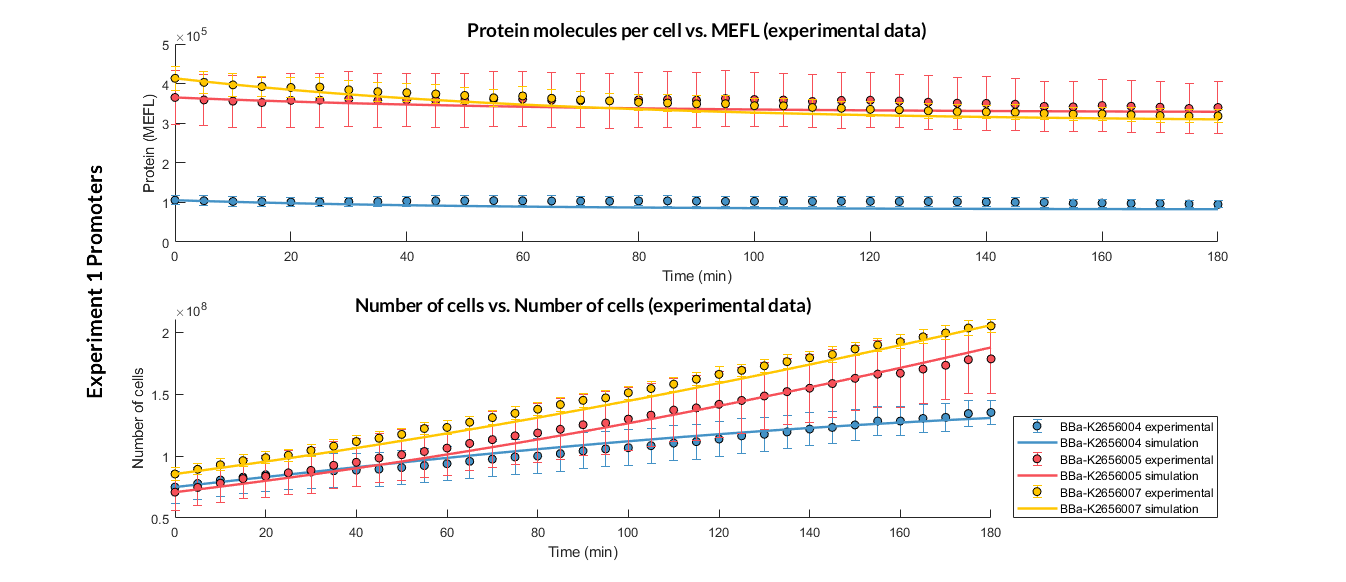
Experiment 1 changing promoters. Experimental and optimized simulated model data of strong, medium and weak promoters.
The results of the graphs have been obtained after an optimization and decision-making process, in which the optimal parameters have been selected and the constituent model for each objective has been simulated and compared with the experimental data. The optimized parameters are summarized in the following table.
Optimized parameters |
Values |
|---|---|
Constitutive transcription rate CR |
|
PoI degradation rate dp |
dp = 0.008492 min-1 |
Dilution rate μ |
|
List of optimized parameters for promoters experiment.
In addition to simulating the optimized models, the Printeria Modeling team has also calculated the relative strength between the different promoters, taking BBa_K2656005 strong promoter as a reference. Likewise, a ratio between CR parameters of the different promoter parts and CR parameter of the reference promoter has been calculated. The characterization of the promoter parts by their relative strength is shown below.
Original BioBrick RBS part |
Printeria RBS part |
Relative strength |
p parameter ratio (pProm/pref) |
|---|---|---|---|
BBa_J23102 (Reference) |
BBa_K2656005 (Reference) |
1 |
1 |
0.9367 |
0.9013 |
||
0.2603 |
0.3172 |
Relative strength between different promoter parts.
In the following experiment we want to compare the degradation rate of different protein reporters in two Printeria TU with identical promoters, RBS and transcriptional terminators. An LVA degradation tag has been added to one of the protein sequences in one TU. This tag causes an increase in protease activity and, therefore, a faster degradation of the reporter protein in the cell. A priori, we can deduce that the degradation rate in the TU that presents the degradation tag will be higher.
With these experiments, our team aims to meet two objectives:
To analyze the effect of the protein degradation rate variation on our constitutive expression model, and determine if the model fits the experimental results of the reporter proteins with LVA degradation tag.
Characterize the YFP reporter protein with LVA tag as a new iGEM part and as Improve project .
The main parameters of the experiment and optimization for each reporter protein are described below. We have followed the usual experimental protocol and multi-objective optimization protocol.
Experiment parameters |
Description |
|---|---|
Time |
06:00:00 (HH:MM:SS). Measurement interval: 05:00 (MM:SS) |
Number of samples |
8 samples for each TU colony |
Number of medium samples |
8 samples of M9 medium |
Temperature |
37 ºC |
Shake |
Double Orbital. Continuously |
Absorbance. Optical Density (OD) measure |
Wavelenght at 600 nm emission |
Excitacion wavelength |
Wavelenght at 500 nm |
Emission wavelength |
Wavelenght at 540 nm |
Gain (G) |
60 |
Biotek Cytation 3 experimental parameters.
Optimization specifications |
Description |
|---|---|
Parameters |
Constitutive transcription rate CR: fixed Translation rate p: to optimize PoI degradation rate dp: to optimize mRNA degradation rate dm: fixed Dilution rate μ: to optimize Maximum growth capacity Kmax: experimental value |
Objetives to optimize |
For each TU, we set 2 objetives: FOD (Fluorescence) and OD (Absorbance). In this experiment we have measured 2 TU, so we are optimizing 4 objectives per experiment |
Parameter ranges |
Constitutive transcription rate CR: [0.01 - 2] min-1 PoI degradation rate dp: [0.0058 - 0.018] min-1 Dilution rate μ: [0.0058 - 0.035] min-1 |
MATLAB files |
spMODEparam.m: it defines the parameters to be optimized, their value ranges, number of objectives, the cost function, the identification and validation experimental data and other spMODE algorithm parameters. When the script is executed, a spMODEDat structure variable is defined. This structure contains all the standardized optimization information that the spMODE algorithm will need for its execution. In this experiment, we have used spMODEparam_exp1YFP.m spMODE.m: it contains the Multi-objective Differential Evolution Algorithm with Spherical Pruning, which optimizes parameters for our experimental results (to execute spMODE.m file we need also SphPruning.m file). CostFunction_improve_RMS_2n.m: it simulates the model with different vector parameters, and calculates the Root Mean Square Error with the identification dataset. Then, it returns the error for each objective and parameter vector. levelDiagram.m: plots Pareto front and Pareto set that gives us back the algorithm. execute_improve_2n.m: this script launches the optimization by executing spMODEparam.m, spMODEm algorithm and levelDiagram.m. Then, allows the user to enter the best parameters, and plots validation experimental data and simulation results in the same graph. |
Optimization specifications for the experiment.
After executing the experiment and the optimization, and selecting the optimal parameters, we obtain the graphical comparison between the experimental and simulated values.
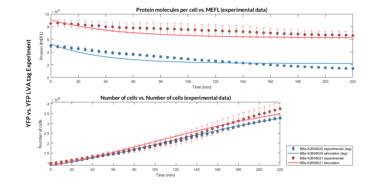
Experiment YFP vs. YFP tag. Experimental and optimized simulated model data of YFP and YFP tag protein
Optimized parameters |
Values |
|---|---|
Translation rate p |
| PoI degradation rate dp |
|
Dilution rate μ |
|
List of optimized parameters.
At this point, it is easy to see that the degradation rate is significantly higher in the reporter protein data with the degradation LVA tag. If we calculate the ratio between the degradation rate of both YFP reporter proteins, we observe that the value of the protein with LVA tag one is about twice the value of the protein without LVA tag.

Inducible expression models
Inducible expression models are those in which the expression of the cell's messenger RNA (mRNA) depends on one or more inducing molecules, which can act as activators or repressors. The concentration of the inducing species determines the level of expression of mRNA and protein in the cell.
Our Printeria device gives us the possibility to create some inducible genetic constructs:
PBAD/araC inducible model
The inducible promoter PBAD/araC [5] is a promoter whose expression depends on two inducing molecules: the L-arabinose (activator) and the araC (repressor). The dimeric protein araC binds to the DNA chain forming a DNA loop and thus prevents the binding between DNA and RNA polymerase. However, when two arabinose molecules bind to the araC dimer, the DNA loop is broken and the binding between the RNA polymerase to the promoting region is possible.
We have proposed a possible mathematical model describing the PBAD/araC mechanism. This theoretical model has been included in the Simulation Tool, so that with Printeria it is possible to predict the behavior of PBAD/araC inducible promoter circuits.
Model design
After analyzing the biochemical functioning of the PBAD/araC promoter, we propose the following cellular scheme that would describe its behavior. It is worth mentioning that we have assumed a very high concentration of araC in the cell, as we have considered that the gene encoding for the araC protein is found in the cell genome (e.g. in DH5α strains).
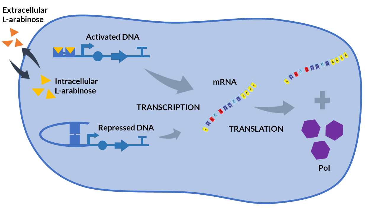
PBAD/araC inducible model. Cell schema.
From the cell schema we can deduce the following biochemical reactions.
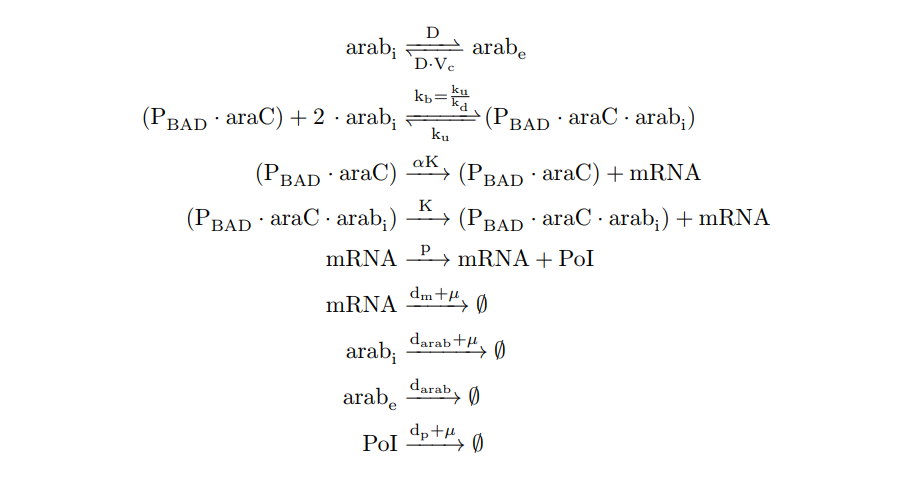
PBAD/araC inducible model. Biochemical reations.
Parameter |
Description |
Units |
Value |
|---|---|---|---|
D |
Diffusion coefficient | min-1 |
2 [2] |
Vc |
Cell volume(1.1x10⁻⁹ μL)/External volume(1x10⁻³ μL) | adimensional |
1.1x10⁻⁶ [2] |
ku |
Dissociation rate of (PBAD.araC.arabi) complex | min-1 |
10 [10] |
kd |
Dissociation constant of (PBAD.araC.arabi) complex | molec2 |
|
kb |
Association rate of (PBAD.araC.arabi) complex. ku/kd | molec-2min-1 |
0.1 (Estimated) |
K |
Transcription rate is the product of transcription rate per plasmid Kt and the mean number of plasmids in cell cn . In our case, we are using the pMBI replication origin, so cn ∼ 500, and K = Kt·cn. |
min-1 |
|
α |
(PBAD.araC) basal activity constant | adimensional |
0.1 (Estimated) |
p |
Translation rate |
min-1 |
2.38 [2] |
darab |
L-arabinose degradation rate. We assume a very slow degradation. |
min-1 |
∼10-6 |
dm |
mRNA degradation rate |
min-1 |
0.247 [7] |
dp |
PoI degradation rate |
min-1 |
0.0063 [5] |
μ |
Dilution rate |
min-1 |
0.017 [5] |
Kmax |
Maximum growth capacity |
cells |
1.6·108 [5] |
PBAD/araC inducible model. Model parameters.
We apply the Law of Mass Action kynetics (LMA) to obtain the differential equations. If we consider that the plasmid copy number cn is constant, we can reduce the model in a differential equation and add an algebraic equation. Thus, we get a model of six differential equations and one algebraic equation, as shown below.
Variable |
Biochemical species |
Units |
|---|---|---|
n1 |
(PBAD.araC.arab) complex |
Molecules |
n2 |
Extracellular L-arabinose |
Molecules |
n3 |
Intracellular L-arabinose |
Molecules |
n4 |
mRNA |
Molecules |
n5 |
PoI |
Molecules |
n6 |
Number of cells |
Cells |
PBAD/araC inducible model. Biochemical species.

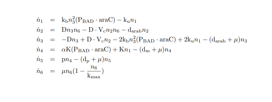
PBAD/araC inducible model. Model equations.
Having developed the equation model from the cell schema and biochemical reactions, we have programmed two MATLAB files: the mi_araC_simplest.m function, which describes the system of differential equations, and the script model_inducible_simplest.m in which the parameters are defined and the model is solved by the ode23t MATLAB function. The result of the simulation of the model is shown below.
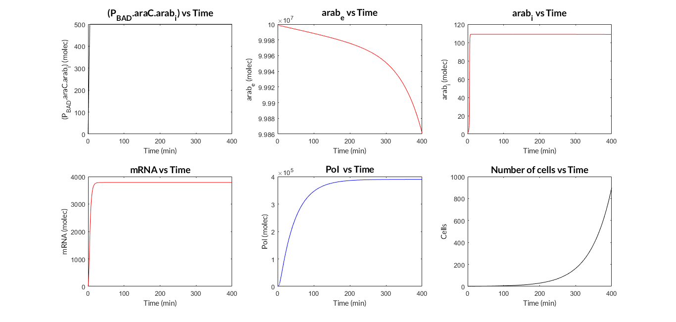
PBAD/araC inducible model. Model predictions using parameter values from literature.
Once the PBAD/araC model is developed and coded, we simulate the model by varying the parameters through our MATLAB script analysis_mi_araC_simplest.m. In this case, we have varied the K transcription and p translation rates and we have represented in a 3D graph the values of the PoI in the steady state.
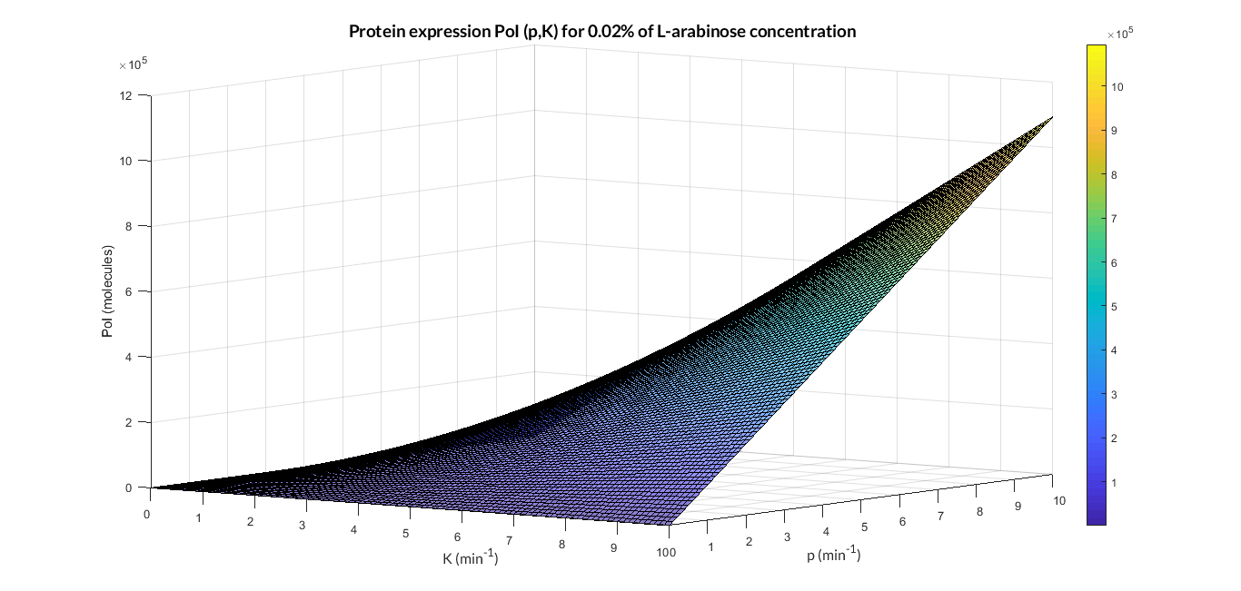
PBAD/araC inducible model analysis. The graph represents de PoI stationary value as function of p and K ratios.
As we can see in the 3D graph, the PoI expression growths exponentially when translation rate p and transcription rate K increase.
But we can also vary the initial concentration of L-arabinose in PBAD/araC model. The set of simulations varying p and arab0 parameters has been programmed in the analysis_mi_araC_simplest_arab.m MATLAB script. We have represented our results of the PoI in the steady state in a 3D graph.
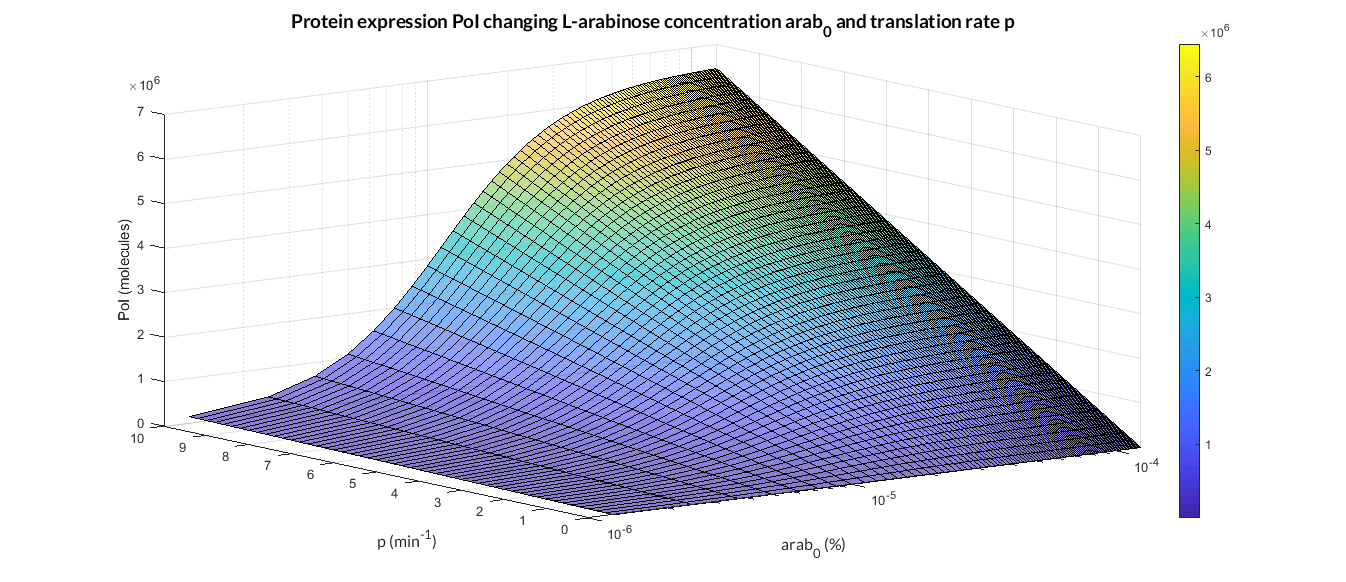
PBAD/araC inducible model analysis. The graph represents de PoI stationary value as function of p ratio and L-arabinose concentration (arab0).
LuxR-LuxI inducible model
RESUMEN DEL FUNCIONAMIENTO DEL CIRCUITO
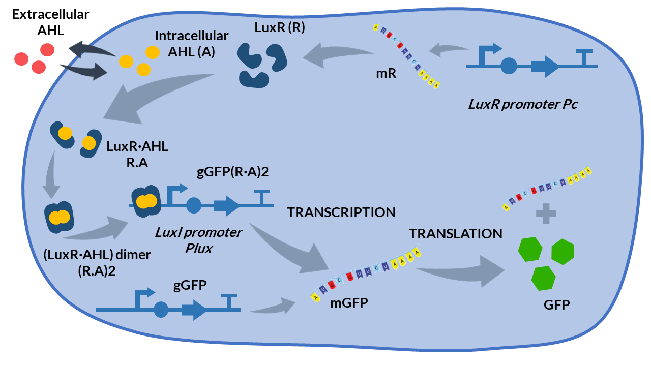
LuxR/LuxI inducible cell schema.
REACCIONES, PARÁMETROS
TABLA DE VARIABLES Y ECUACIONES
Analisis
Multi-objective parameter optimization
To what extent is our model valid? What values should the parameters take? To what extent do the theoretical results resemble the experimental ones? Is our model able to explain the behaviour of cells in reality?
One of the most important phases in the field of Printeria Modeling has been the validation of theoretical models with experimental data. In the Printeria team we wanted to confirm that the models designed are consistent with our experiments. However, we know that the parameters will not take a fixed value, but vary depending on the genetic construction with which we experiment. With this idea in mind, the need to apply an optimization process arises.
The process of multiobjective parameter optimization [3] consists in minimize two or more design objectives that have a trade-off between them as function of some decision variables. In our case, these objectives are estimation errors between experimental data and model predictions, and the decission variables are some of our model parameters. From a dataset, and applying a mathematical algorithm, we can find the optimal solutions, also known as Pareto-optimal. These optimal solutions are such that there are no more solutions that do not improve one objective without worsening the rest.
As this is a multi-objective optimization, there is usually no single optimal solution, but rather a set of them which form the Pareto front. For each of these solutions, we find a set of decision variables associated: the Pareto set[6]. In our case, the Pareto front solutions represent the RMS error between experimental data and simulations, and the Pareto set is the set of parameters that give rise to these solutions.
From the Printeria Modeling team we have established a protocol that allows us to obtain the optimal solutions of the model parameters for any experiment:
We define the objectives to be optimized. These will be the values of Fluorescence F/Unit of Absorbance OD or FOD, and the cellular growth (OD) of a Transcriptional Unit (TU). Therefore, if we have different n TU in an experiment, we will optimize 2n objectives.
We choose the parameters to optimize and establish the range of values they can take.
We select the identification and validation data. The identification data are those used in the optimization process. The validation data are used to compare the experiment with the simulated theoretical model and the optimized parameters.
We define the cost function, which specifies the error function to be minimized, simulates the model with different parameter values, and calculates the error between the simulation data and the experimental identification data.
The mathematical optimization algorithm is executed. In our case we use the Multi-objective Differential Evolution Algorithm with Spherical Pruning. This algorithm uses the cost function to test different parameter values and thus search for optimal parameter values.
The Pareto set and Pareto front diagrams and the different solutions of our optimized parameters for the different objectives are obtained.
Decision Making is carried out by the designer. The optimal parameters are chosen for our 2n objectives.
The model is simulated with the optimized parameters and compared with the validation data.
Following this protocol, and particularizing it for each experiment, we have been able to determine the validity of our models and obtain the best parameters for our experiments.
Simulation Tool
One of the main challenges of the Printeria project has been to give the user a chance to really understand what our device is doing when it prints genetic circuits on bacteria. Facing this challenge, we have also sought to provide as much information as possible about the Printeria product. And what better way than to give our user a quantitative, mathematical description of what happens in our cells?
In our project we believe that mathematical modeling can be a very powerful tool for transmitting knowledge, so the Printeria Software and Modeling teams have brought together the most outstanding mathematical models in a single Simulation Tool.
Our Simulation Tool has been conceived as a mathematical model simulation program that has been perfectly integrated into our Printeria Controller software. When our user wants to assemble a genetic construct and selects the parts, the Simulation Tool offers the possibility to experiment in silico and predict cell behavior before printing the bacteria. All this, just by pressing the Show model results button... and instantly!
But how does the Simulation Tool work?
The Printeria Modeling and Software teams have jointly designed a program developed in a single Python script (have a look at our simulate.py script). The program combines the functions of the main mathematical models of Printeria with the information of the Printeria kit stored in the Printeria database. In addition, as it is a single Python file, it is stored and run on the Raspberry Pi 3 server.
Now let's see what happens if the user has chosen the Printeria parts and presses the Simulate button...
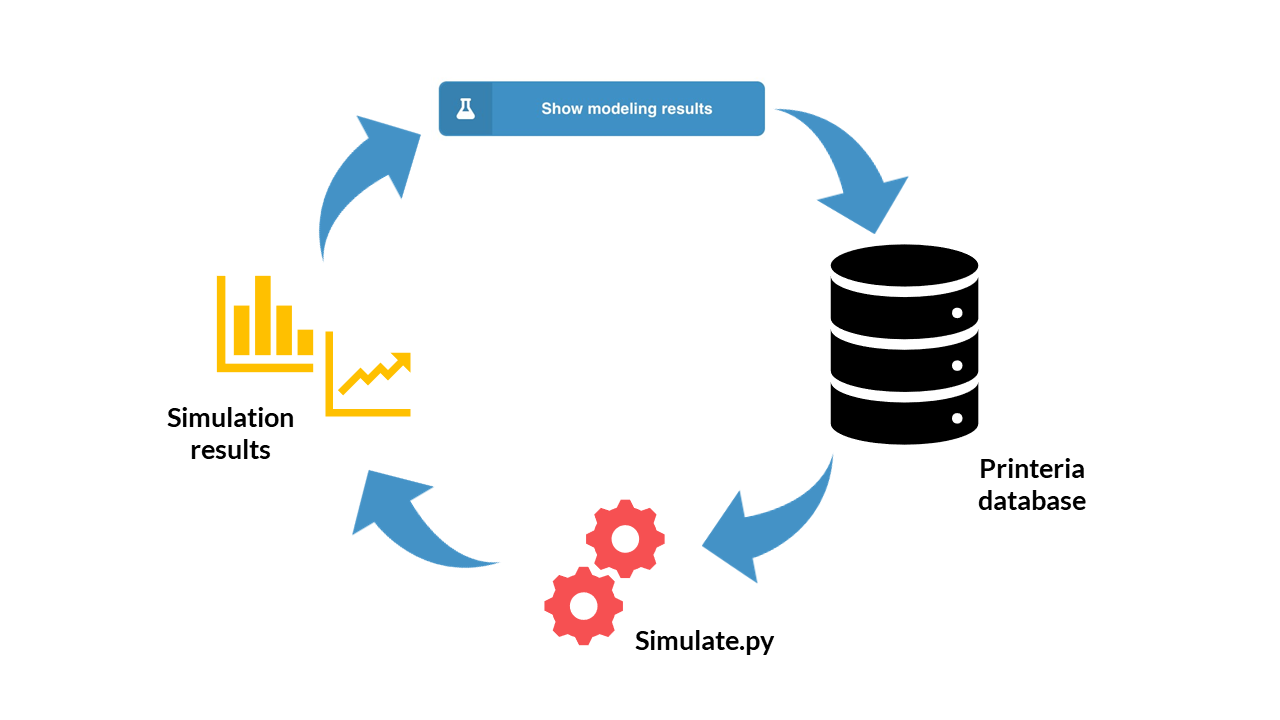
Simulation Tool working scheme.
The Printeria client connects to the Printeria MongoDB database where we store all the information of our Printeria kit.
The four parts of the genetic construction (promoter, RBS, CDS and transcriptional terminator) are extracted from the database thanks to their identifiers.
The type of model (constitutive or inducible expression) is identified from the type of promoter selected.
The model parameters of each construction part are extracted.
The initial conditions of the simulation and its duration are established.
The model is simulated using Python's odeint function
A temporary CSV file is generated in which the we store the results of the simulation in a certain format.
From the CSV file, the simulation results are represented graphically on the Printeria site. The user can view or download their results.
And what are the advantages of an application like our Simulation Tool?
User-friendly. It is very simple to operate for the user. Just select your Printeria parts, press a button... And that's it!
Integrated. All our software is included in the Raspberry Pi 3 server. You don't need to download the program.
Instant experimental data. Our Simulation Tool runs simulations at high speed. In a few seconds you'll have your results.
Customizable parameters. You can modify your parameters and adapt them to your experiment, to obtain more precise results.
All-in-one. Our Simulation Tool includes several mathematical models, constitutive and inducible, in a single code and solves them particularizing for each Printeria genetic construction.
Would you like to try the Simulation Tool? Go to our Printeria Controller site and discover all the possibilities offered by our software.
What are you waiting for to start discovering it?
References
Picó, J., Vignoni, A., Picó-Marco, E., & Boada, Y. (2015). Modelado de sistemas bioquímicos: De la ley de acción de masas a la aproximación lineal del ruido. Revista Iberoamericana de Automática e Informática Industrial RIAI, 12(3), 241-252.
Y. Boada, A. Vignoni, and J. Picó. Engineered control of genetic variability reveals interplay among quorum sensing, feedback regulation, and biochemical noise. ACS Synthetic Biology, 6(10):1903–1912, 2017a.
Segel, L. A., & Slemrod, M. (1989). The quasi-steady-state assumption: a case study in perturbation. SIAM review, 31(3), 446-477.
Boada, Y., Vignoni, A., Reynoso-Meza, G., & Picó, J. (2016). Parameter identification in synthetic biological circuits using multi-objective optimization. Ifac-Papersonline, 49(26), 77-82.
R. Milo and R. Phillips. Cell Biology by the Numbers. First edition, 2015. ISBN9780815345374.
Boada, Y., Vignoni, A., & Picó, J. (2017). Reduction of population variability in protein expression: A control engineering approach. Actas de las XXXVIII Jornadas de Automática.
U. Alon. An Introduction to Systems Biology. Desing Principles of Biological Circuits. Champan and Hall/CRC, Edition, 2007.
Schleif, R. (2000). Regulation of the L-arabinose operon of Escherichia coli. Trends in Genetics, 16(12), 559-565.
Boada, Y. (2018). A systems engineering approach to model, tune and test synthetic gene circuits. PhD. Thesis, Universitat Politècnica de València.
N. E. Buchler, U. Gerland, and T. Hwa. Nonlinear protein degradation and the function of genetic circuits. Proceedings of the National Academy of Sciences of the United States of America, 102(27):9559–9564, 2005.