Team:SUSTech Shenzhen/Model
Overview &formulation
In our wet lab experiments, we developed a novel Two-Cell system to study cell-cell communication. Millions of donor cells with single gene alteration convey the signal to the receptor cells, according to the response of receptor cells, we can back to investigate the alterations of interest.
However, the fantastic engineering approach does have some limitations, first, when future iGEM teams move further to design larger screening, like whole genome screening, our initial methodology of capturing two cells within one droplet could potentially become less applicable, because of cell death during the long emulsion time. Nevertheless, this drawback can be overcome by further improve our hardware, also, the reverse approach by modeling may open up a new window. We can use pre-existing knowledge and bioinformatic method to narrow down the screening size previously.
Another thing we found in experiments is the Wnt response capability of Wnt receptor cell is weak and it needs time to send out response. Then, we wanted to see is it possible to use computational modeling to simulate the biological process of Wnt signaling and help to optimize experiments.
And we can never work with an engineered system without any quantification, that will largely blot out our understanding of our engineered system. So, we want to build a encapsulation model from our own experimental data to see whether we can improve our system from theoretical perspective.
So, for modeling, we have three aims:
1
Narrow down the screening size and explore potential secretion-related candidate genes through co-expression analysis.
2
Define the importance of key features in signaling pathway to optimize our construction of receptor cell.
Before any biological modeling, the most important thing is formulating the scenario, and for these secretion and reception can be regarded as two systems, one secret Wnt after a cellular process, the other give response after signal process. (Fig1)
After simplification, the diagram is like Fig2. For the right part, Wnt gene as the origin, known or unknown factors influencing the process to mature Wnt protein. For the left part, Wnt protein becomes the input. And the output is Wnt pathway target genes.

Figure1. Real scenario of Wnt pathway.

Figure2. Formulated diagram of Wnt pathway.
Genes prediction model of Wnt secretion
For Wnt secretion part, we want to use co-expression analysis to search Wnt secretion-related candidate genes to narrow down our screen size o f gRNA library. This means we use these known factors, which are known enzymes involving in Wnt protein maturation, like PORCN and WLS, to fish new unknown factors.
And the basic principal of co-expression of two genes is shown in Fig 1, it compares the expression patterns of two genes across samples, define their co-expressing correlation valves. The higher the valve, the more similar they are, they may undertake the same function. (Zhang, et al, 2005) And once we get the co-expressing gene list, we can design a more specific gRNA library to do engineered screening.

Figure3. basic principle of co-expression of genes
The co-expression model is based on Pearson correlation coefficient between two genes. The formula is shown as below in Fig4.

Figure4. The formula of Pearson’s correlation coefficient. xi and yi are two genes’ expression level index with i. n is the sample size. ¯x is the mean expression level of all samples, and analogously for ¯y.
We have collected a large amount of gene expression datasets of different samples from online databases (Dam, et al, 2014), we regarded it as n samples. And for each sample, it consisted of a large gene list which couples with their expression level. We regarded it as m genes. Therefore, it’s a m x n matrix, for the expression pattern of each gene, it’s actually a n dimension vector. Pearson’s correlation coefficient measures the tendency of these two vectors of gene expression level to increase or decrease together, giving a value of their overall correspondence.

Figure5. The pipeline of heatmap generation
After calculating Pearson’s correlation coefficient of each pair of genes from expression matrix, we generate a correlation matrix. And we apply heatmap to present the results (Fig5), each column is one sample’s gene expression, each row is one gene’s expression level across samples. The genes with high Pears on’s correlation coefficient cluster together automatically, so do the samples. (Fig6) Then, we focus on the gene cluster around our reference genes, PORCN and WLS.

Figure6. Part of a small heatmap generated from gene expression matrix. (18 samples only) Each column shows one sample’s gene expression; each row shows one gene’s expression level across samples. WLS is in highlighted color. (data from NCBI, Schoumacher, et al, 2014)
After a series heatmaps were generated, we extract two gene lists based on the workflow diagram of Fig7. We compare each genes’ coefficient with WLS, rank them, set a threshold, select out the genes with coefficient larger than threshold to obtain a new list, in which every gene is considered as potential related genes to WLS. Because we have lots of samples actually, which will intrinsically to get lower Pearson’s correlation coefficient as the dimension of vectors of gene expression gets higher. Therefore, final Pearson’s correlation coefficient we get is different from Fig5 shows, which only contains 18 samples. They are no more than 0.7.

Figure7. Workflow diagram of potential gene selection. (WLS as an example.)
So, for WLS related genes, we set the threshold as 0.3, through which we get 215 genes. And for PORCN related genes, we set the threshold as 0.25, through which we get 108 genes. Top10 genes and their annotations are shown in Table1 and Table2. From these two tables, we can see even the sample size is large, we can always get some highly related genes. However, from the annotations of these potential genes, we can not draw a strong conclusion without further verification. This point does reveal the complexity of biological phenomena. There is even an uncharacterized gene that has high correlation coefficient with PORCN. Besides their annotated functions, these genes may have potential relation to WLS and PORCN, and they may play roles in Wnt secretion pathway.
Table1. Top10 related genes to WLS generated from correlation model. Annotations show the validated functions of genes.

Table2. Top10 related genes to WLS generated from correlation model. Annotations show the validated functions of genes.

Now that we have two potential Wnt secretion-related gene lists, but we are still uncertain to say they are related to Wnt secretion. In order to further verify the results, we can use these gene lists to narrow down our gRNA library and screening size, then use our engineered system to perform double emulsion experiments, hopefully, we can verify these genes with high efficiency.
On the other hand, we try to further narrow down the size of these two gene lists to find out the candidate genes through modeling. First, we merge these two lists to form one gene list. And then the improving method is identifying the differentially expressed genes between Wnt high secretion cell and Wnt low secretion cell. The intersection of these differentially expressed genes and our previous co-expressed genes should have much higher potential to be Wnt secretion-related genes.
Kinetic model of Wnt signaling
For the left part of Fig1 and Fig2, we wanted to define the importance of key features in signaling pathway to optimize our construction of receptor cell line. The changes of output can be regarded as accumulation of the changes of input and pathway components. Obviously, the change of input (Wnt ligand) contributes the most to the whole signaling pathway. However, when we fix the Wnt ligand, how much do the other components contribute?
To answer this question, we integrated our experimental observation and data pre-existing knowledge (MacDonald, et al, 2009; Clevers, 2006; Anastas & Moon, 2013), and gene expression data from online database[TCGA, 2012] to deeply analyze Wnt signaling pathway, then construct a contribution model to update our understanding of this pathway. Once we know the contribution coefficient, we can adjust the signaling pathway through knock down or overexpression experiments to make the reception cell more sensitive.
Wnt signaling pathway is presented on the KEGG database (Kanehisa, et al, 2000) and Pathway-Common (Cerami, et al, 2010). We picked genes from Wnt canonical pathway according to previous researches as our pathway components. Also, some useful information was found on GTEx, TCGA and NCBI databases, including gene expression data and gene description.
Finally, we collected the gene expression data of 50 different normal samples. And we have selected one input gene, WNT2, one output gene, C-MYC, which is one of WNT pathway targets, and x component genes, they are SFRP, DKK1, LRP5, LRP6, FZD2, BAMBI, DVL1, DVL2, DVL3, GSK3B, APC, AXIN1, CTNNB1, CSNK1A1, TCF7, C-MYC. Besides, in order to test the feasibility of our method in the last procedure, we introduced three control genes, they are: CFL1, NPM1, CALR. All of them are housekeeping genes, which means their expression keeping in a relatively stable level and have no effects on Wnt signaling pathway.The picture of formulated wnt canonical signaling pathway including our selected genes is shown in Fig8.

Figure8. Formulated wnt canonical signaling pathway. Rounded rectangle represents components in signaling pathway, oval represents input and output.
After a series of essential formulation done, we began our real modeling.
Step1. Data Pre-processing
Purpose: To make sure all the sample under the similar WNT exposing condition, to fix Wnt ligand input.
In the beginning, we used grey relation analysis (GRA) to select the samples that under the same physiological condition, which means they should possess the same extracellular environment. GRA is one kind of methods to describe curves similarity quantitively. Fig9 explains how it works.

Figure9. Example of Grey Relation Coefficient, the more similar two curves are, the higher GRA coefficient they have.
We chose the first sample as our reference sample and calculate the grey relation coefficient of the other 49 samples compared to the first sample. The results are represented as distribution histogram (Fig10). After that, normal function was applied to fit it. Result shows all samples are under very similar condition. All of them can be used in our following processes.

Figure10. The standardized results of grey relation analysis.
Step2. Cluster Analysis
Purpose: Pre-define some correlation parameters based on pre-existing gene connections.
For gene pathway analysis, it’s very common to use cluster analysis to verify the connection between genes. In order to better simulate their inner relationship, we chose hierarchical clustering as our analysis method.
We possessed 50 samples’ gene expression data, after filtering, each sample contains 17 genes that we are interested. This indicates a 17 × 50 matrix. Each gene is a 50 dimension vector. If we normalize it and calculate the distance between each pairs of genes, an 17 × 17 distance matrix will be generated. We picked out the gene pair that has the smallest distance and put them all together, their average valve will be treated as a new column. Then, calculate the distance again and find another pair, repeat it until we cluster them all. Our cluster result are as shown in Fig11.

Figure11. The clustering result for our selected genes
It’s very surprised for us to get this result. As the figure shows, DVL1/2/3 are clustered together, the distance between LRP5 and LRP6 is also very small. Moreover, their relationship is nearly coincided with the canonical pathway of Wnt signaling. This result further encouraged us to continue. The distance between genes was then extracted and used in the following step.
Step3. Pathway Analysis
Purpose: Define the contribution strength of pathway components
The relationship between genes is very complex and the basic assumption here is every two genes are linked. The concrete interactive network is under the mist through. These complicated effects include but not limited to: feedback regulation, transgenic interaction, coexpression effect.
It’s important to quantify these all effect in one form. Correlation coefficient is the basic math analysis method, which reveals their mathmatic relationship in a total black box. The correlation coefficients between of our selected genes were calculated. Results are as shown in Fig12.

Figure12. The correlation coeficient matrix between selected genes.
However, a single correlation coefficient will cause lots of error. Combing with the cluster, which reveals genes relationship in a relatvie accurate way. We modified correlation with their distance data and normalize it. This is the new correlation coefficient for unknown relationships. While for those known gene relationships, we modify it manually according to the previous results.
Let’s back to our assumption: Every two genes are linked. It’s necessary to say: The strength of the link was quantified by modified correlation coefficient.If every two genes are linked, it means one gene can cause some effect on all other genes through many pathways.
Considering component gene A, B, C and output gene. If we want to calculate the effect caused by A. Here are five conditions:
- A → output
- A → B → output
- A → C → output
- A → B → C → output
- A → C → B → output
If we calculate one gene acts on output through 1 gene. We need to solve the equation below to find out direct pathway coefficient:

As the formula shows, p is the direct pathway coefficient and r is the correlation coefficient. Due to the limitation of the computing power, we can’t list all possible ways. Nevertheless, it’s enough for us to calculate one gene acts on output through 4 genes. (Correlation coefficient is always less than 1, more than 4 genes connection can be ignored.)
We solve the equations and find out P value for each pairs of component gene to output gene(C-MYC). P is treated as direct effect from genes to Wnt signaling pathway. The final results are shown in the Fig13.
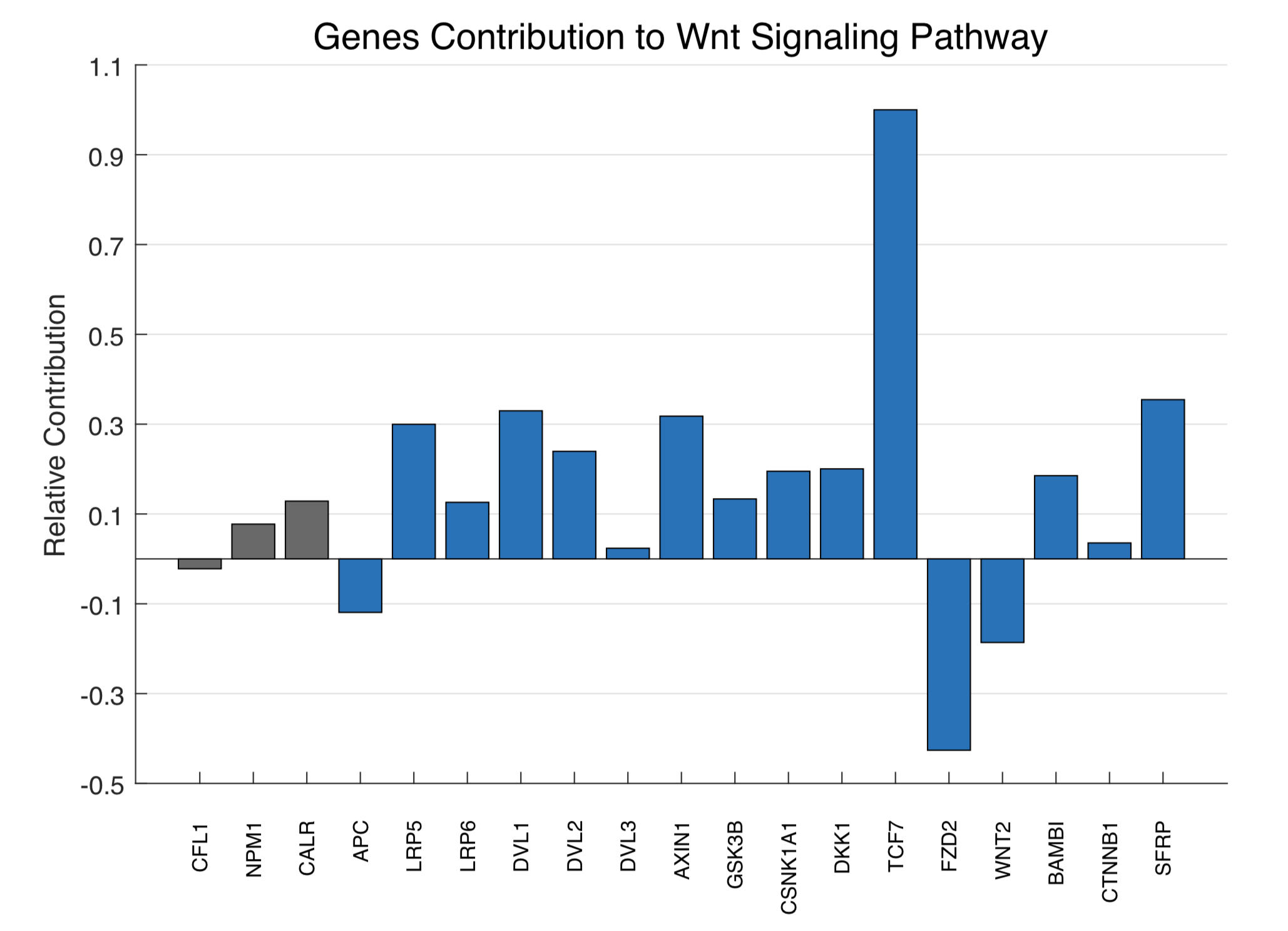
Figure13. Genes contribution to Wnt signaling pathway based on pathway analysis
As the result shows, our control genes are at a low level around zero, which means they do not affect too much. They do have a value can reflect the systematic errors of our methods. The TCF7 was the biggest contributor to Wnt signaling pathway. Nevertheless, other genes effects are still very close to known pathway relationship, which reveals the correctness of our methods.
And the results actually can help us construct our reception cell line, to adjust the condition of signaling pathway so as to maximize the sensitivity of Wnt response.
Model of encapsulation
Since we apply the double emulsion system to encapsulate the cells, we want to estimate the efficiency of the system. That is, we aim to deduce the total time in which the required cells are encapsulated.
The experience of experiments tells us that the number of particles containing in one droplet obeys the Poisson
Distribution. Hence, the first step is to estimate the coefficient of the distribution. Assume refers to the number of particles containing in droplet
 and
and .
Then the moment estimator of
.
Then the moment estimator of is
is . After many times of trials with single channel feed, we conclude that
 . Hence, we are able to draw the distribution
probability of single channel feed. (Fig14)
. Hence, we are able to draw the distribution
probability of single channel feed. (Fig14)

Figure14. Particle number distribution of single channel feed.
With the condition of double channel feed, we assume the two feeding channels are independent and the new Poisson Distribution follows . Then we are able to draw the distribution probability of double channel feed. (Fig15) As we can see, the probability of two particle encapsulated in one droplet is 1.64%. That means if 10000 droplets are produced, about 164 of them are exactly what we need.

Figure15. Particle number distribution of double channel feed.
The second step is to optimize the droplet generation rate. With larger droplet generation rate (The number of droplets produced per second), less time is required to produce the sample. We denote the Droplet Generation Rate as DGR, the number of the encapsulated cells required as N, the Poisson Distribution with single channel feed as , the Poisson Distribution with double channel feed as . Then the required time is calculated by the formula in Fig16.

Figure16. The formula of requiring time.
And we draw the graph of the above function, DGR as x-axis and required time as y-axis. (Fig18) We can infer from the graph that the time required is inverse proportional to DGR. When DGR is large than 3500, the time changes little. Hence, we may modify the system where DGR is around 3500 to make it more effective.

Figure17. The graph of function in Fig16, required time vs. DGR.
Discussion
Our modeling and analysis are all based on scientific logic, real data, and literature conclusion, we are focusing on the improvement and complement for our experimental design and engineered system. Also, both the co-expression methods to narrow down screen size the optimization methods for reception cell line are able to give considerations and inspirations for future iGEM team that wants to extend our ideas, designing more exciting projects related to intercellular communication. What’s more, the simulation model of double emulsion system can provide ways to make it more applicable for other teams and other fields. We do look forward to seeing it is applied to various fields, like biosensor, biosynthesis and drug screening.
References
Zhang, Bin and Horvath, Steve (2005) "A General Framework for Weighted Gene CoExpression Network Analysis," Statistical Applications in Genetics and Molecular Biology: Vol. 4: Iss. 1, Article 17. DOI: 10.2202/1544-6115.1128
van Dam, S., Craig, T., & de Magalhaes, J. P. (2014). GeneFriends: a human RNA-seq-based gene and transcript co-expression database. Nucleic acids research, 43(D1), D1124-D1132.
Schoumacher, M., Hurov, K. E., Lehár, J., Yan-Neale, Y., Mishina, Y., Sonkin, D., ... & Cooke, V. G. (2014). Inhibiting Tankyrases sensitizes KRAS mutant cancer cells to MEK inhibitors via FGFR2 feedback signaling. Cancer research, canres-0138.
Anastas, J. N., & Moon, R. T. (2013). WNT signalling pathways as therapeutic targets in cancer. Nature Reviews Cancer, 13(1), 11.
Clevers, H. (2006). Wnt/β-catenin signaling in development and disease. Cell, 127(3), 469-480.
MacDonald, B. T., Tamai, K., & He, X. (2009). Wnt/β-catenin signaling: components, mechanisms, and diseases. Developmental cell, 17(1), 9-26.
Cancer Genome Atlas Network. (2012). Comprehensive molecular characterization of human colon and rectal cancer. Nature, 487(7407), 330.
Cerami, E. G., Gross, B. E., Demir, E., Rodchenkov, I., Babur, Ö., Anwar, N., ... & Sander, C. (2010). Pathway Commons, a web resource for biological pathway data. Nucleic acids research, 39(suppl_1), D685-D690.
Kanehisa, M., & Goto, S. (2000). KEGG: kyoto encyclopedia of genes and genomes. Nucleic acids research, 28(1), 27-30.
©2018 SUSTech_Shenzhen
